# Install packages if not already available
install.packages(c(
  "glmmTMB", "lme4", "DHARMa", "performance", "parameters", "ggplot2",
  "dplyr", "gridExtra", "knitr", "catdata"
))1 Introduction
In the past couple of years, I have worked with many healthcare datasets containing large numbers of zero outcomes. This problem is not unique to healthcare: in fact, it spreads across many fields including ecology, insurance, consumer behaviour and so on. When this is the case, it can make standard count models difficult to apply – Zero-inflated models can offer one flexible way to circumnvent this issue.
That flexibility also makes these models harder to implement and interpret, and they receive less attention than many other machine-learning algorithms, so I initially found it difficult to locate practical guidance that connected the theory, code, diagnostics, and interpretation.
This tutorial grew out of the notes I made whilst applying zero-inflated models in industry, and of the internal training sessions I later ran on the topic. My goal is to provide a practical, hands-on guide to understanding and implementing zero-inflated models. There is some theory involved, but no background on this topic is necessary: the article builds up from ordinary count regression before introducing the two-process model.
This tutorial covers the theoretical foundations, practical implementation, model comparison, diagnostics, and interpretation of some of the simpler and more common zero-inflated count models. In the future, a follow-up tutorial may examine hurdle models, alternative count distributions, and more advanced validation strategies!
In terms of tooling, I strongly recommend the glmmTMB package in R, which is flexible, widely adopted, and well suited to the generalized linear model extensions used here. The Python ecosystem for this task is not quite as mature yet, although for standard applications the statsmodels library is a good starting point. The modelling sequence in this tutorial is simple enough and should be easily transferable if you decide to take that approach.
1.1 What Are Zero-Inflated Models?
In classical statistical regression terminology, zero-inflated models are defined by combining two components: a point mass at zero and a second distribution for the outcome. This essentially means that predictors can enter both components through separate linear predictors and link functions. In this sense, zero-inflated regression models are considered generalized linear mixture models.
Although they are often introduced for count data, the general framework is not limited to counts. For example, Liu et al. (2019) review zero-inflated models for non-negative continuous outcomes, while Ospina and Ferrari (2012) develop zero-or-one-inflated beta regression for proportions.
For the sake of simplicity, this tutorial will focus on count data, where an observed count can arise from two distinct latent processes:
- A latent extra-zero state, whose zeros are often called structural zeros.
- A count-generating state, which produces sampling zeros as well as positive counts.
What does this actually mean? Well, suppose you are modelling how many visits a GP clinic receives over time. Now, a potential patient registered to the clinic in the local area may or may not actually visit during the study period. A zero can mean at least two different things:
- the person was never really in a position to generate a visit during the study window
- the person could have generated a visit, but happened not to
A zero from the first route is called a structural zero; one from the second is a sampling zero. A standard one-process count model, such as Poisson regression, treats both people as coming from the same count-generating process. A zero-inflated model represents both routes as latent possibilities, but the data do not reveal which route produced any individual zero.
1.2 When Do We Need Zero-Inflated Models?
The key challenge zero-inflated models try to address is excess zeros in the data. However, the useful question is not “does my dataset contain a lot of zeros?”, but do the zeros plausibly come from more than one process?
This distinction will become clearer in the following sections, but for now these are some helpful examples to keep in mind:
- Healthcare use: Some patients are effectively unable to generate events because they never access services (structural zeros)—for example, people living in remote areas with no nearby clinics, or those excluded by policy or eligibility criteria. Other patients could use services but happen not to during the study window (sampling zeros)—for example, healthy patients who simply do not visit in that period or patients whose condition does not require care.
- Disease surveillance: Some locations truly have zero prevalence for a pathogen because the pathogen cannot survive there or has been eradicated (structural zeros). Other locations harbor the pathogen but a given survey fails to detect it during that sampling round (sampling zeros) — e.g., low prevalence or imperfect tests.
- Specialist treatments or prescriptions: Some patients will never be eligible for a specific specialist-only procedure or advanced drug (structural zeros) — think of treatments restricted by age, comorbidity, or insurance coverage. Other patients are eligible but simply don’t receive the treatment during the study window (sampling zeros) because they don’t yet need it, they defer care, or the treatment is rarely used in short follow-up.
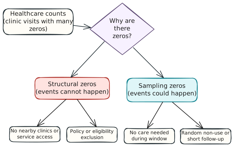
In each case, the zero may carry information about the process that generated the observation. That still leaves an important modelling caveat: excess zeros are not the same thing as proven structural zeros. A flexible one-process count model can sometimes reproduce many zeros without needing a separate latent class.
2 Theoretical Foundation: From GLMs to Mixture Models
2.1 Generalized Linear Models
Before fitting zero-inflated models, it helps to revisit what and how generalized linear models (GLMs) work. If you are already familiar with them, you may want to skim this section or jump directly to Section 3; otherwise, this section provides a concise refresher.
Counts are non-negative integers, usually right-skewed, and often have variance that changes with the mean. Ordinary linear regression is not able to encode those features well: it can predict negative values, and it assumes a constant-variance normal error structure. GLMs are a flexible framework that allow us to retain a regression-style mean model while using a response distribution suited to the outcome.
A GLM connects a linear predictor to the mean of an outcome distribution through a link function. Three ingredients define that structure:
- Linear predictor (\(\eta_i=X_i\beta\)): a linear combination of predictor values and coefficients
- Link function (\(g(\mu_i)=\eta_i\)): the transformation connecting the linear predictor to the conditional mean
- Response distribution: a distribution suited to the outcome, such as Bernoulli for a binary response or Poisson for a count
This recipe is what defines a model of this class, and you can see in Figure 2 how the components relate to one another:

Zero-inflated count models use this structure twice: a binary component models membership in the latent extra-zero group, and a count component models the expected outcome among observations in the count-generating group. The original zero-inflated Poisson regression paper framed this as a practical way to model excess zeros in manufacturing defects (Lambert 1992); the same idea now appears across health, ecology, insurance, and many other settings.
For a simple Zero-inflated model, Logistic and Poisson regression are usually the two building blocks, as we will later see. For now, a short exponential-family refresher first recovers the logit link for a Bernoulli response, and the following count-model section then applies the same logic to Poisson regression and its extensions.
2.2 The Exponential Family
The exponential family is a collection of probability distributions with a shared mathematical form. This might sound abstract, but it includes most distributions you encounter in practice: normal, poisson, binomial, gamma, and many others.
A density or probability mass function in this family can be written as:
\[f(y\mid\theta, \phi) = \exp\left\{\frac{y\theta-b(\theta)}{a(\phi)} + c(y,\phi)\right\}.\]
The notation separates the parts that govern the distribution:
- \(\theta\) is the natural parameter;
- \(\phi\) is a dispersion parameter, with \(a(\phi)\) controlling its scale;
- \(b(\theta)\) determines the mean and variance through its first two derivatives;
- \(c(y,\phi)\) supplies the remaining terms needed to define a valid distribution.
Even though the formula looks daunting, the important part to keep in mind is that this format essentially standardises how we work with different distributions. In particular, it can be proved that for all distributions in this family, the mean and variance are:
\[E(Y)=b'(\theta), \qquad \operatorname{Var}(Y)=a(\phi)b''(\theta).\]
This common structure is what allows GLMs to pair different response distributions with a linear predictor! 1
2.2.1 The Bernoulli Distribution
For a Bernoulli outcome \(Y\in\{0,1\}\) with success probability \(p\),
\[f(y\mid p) = p^y(1-p)^{1-y} = \exp\left\{y\log\left(\frac{p}{1-p}\right)+\log(1-p)\right\}.\]
Writing the mass function this way identifies the natural parameter as
\[\theta=\log\left(\frac{p}{1-p}\right),\]
also known as the logit of \(p\). Bernoulli regression therefore uses the canonical logit link:
\[\operatorname{logit}(p_i)=\log\left(\frac{p_i}{1-p_i}\right)=X_i\beta.\]
The linear predictor \(X_i\beta\) can take any real value, while the inverse-logit transformation keeps \(p_i\) between 0 and 1.
Exponentiating a coefficient gives an odds ratio: \(e^{\beta_j}\) is the multiplicative change in the odds for a one-unit increase in \(x_j\), holding the other predictors fixed. For example, if \(\beta_j=0.20\), then \(e^{0.20}=1.22\), corresponding to a 22% higher odds for a one-unit increase in \(x_j\). We will later use this same link to model the probability of latent extra-zero membership.
Changing the response distribution changes the canonical link and the variance assumption, but not the basic GLM architecture. We now make that transition from a binary response to a count response.
2.3 Count-Model Building Blocks
Poisson regression is the count-data counterpart to the Bernoulli example above: its exponential-family form produces a log link, while its response distribution supplies the mean-variance relationship. This separation is important because the link and the variance assumption can succeed or fail for different reasons.
In the practical section, we will start with Poisson regression and check whether it can account for the variation and the number of zeros in the data. If it cannot handle the variation, we’ll try negative binomial regression, which allows for a more flexible variance structure. Then we can see whether adding a separate zero-inflation process helps. This is also the approach that I recommend taking when tackling real-world data.
2.3.1 Poisson Regression
Poisson regression is usually the standard first model for a count outcome. For person \(i\), it assumes
\[Y_i \mid X_i \sim \operatorname{Poisson}(\lambda_i), \qquad \log(\lambda_i) = X_i\beta.\]
Its probability mass function has the exponential-family form
\[P(Y_i=y\mid X_i)=\frac{\lambda_i^y e^{-\lambda_i}}{y!} =\exp\left\{y\log(\lambda_i)-\lambda_i-\log(y!)\right\}.\]
The natural parameter is therefore \(\theta_i=\log(\lambda_i)\), with \(b(\theta_i)=e^{\theta_i}=\lambda_i\). The canonical log link keeps the expected count \(\lambda_i\) positive. Here, exponentiating a regression coefficient gives a rate ratio: if \(\beta_j=0.20\), then \(e^{0.20}=1.22\), corresponding to a 22% higher expected count for a one-unit increase in \(x_j\), holding the other predictors fixed. Notice how the interpretation is different from the odds ratio in the Bernoulli case: an odds ratio of 1.22 changes a 10% event probability to about 11.9%, whereas a Poisson ratio of 1.22 changes an expected count of 10 to 12.2.
The Poisson distribution has no estimated dispersion parameter, so \(a(\phi)=1\) in the general exponential-family form. Its derivative relationships are therefore
\[ a(\phi)=1, \qquad b'(\theta_i)=b''(\theta_i)=e^{\theta_i}=\lambda_i, \]
and hence the Poisson mean–variance relationship
\[ E(Y_i \mid X_i)=\operatorname{Var}(Y_i \mid X_i)=\lambda_i. \]
This equality applies after conditioning on the predictors. Across the sample, people can have different values of \(\lambda_i\), so combining their count distributions can produce a raw variance larger than the raw mean even when the conditional Poisson assumption holds. A large variance-to-mean ratio or a large number of zeros is therefore a warning, not evidence by itself of either conditional overdispersion or a separate zero-generating process. We assess those possibilities after fitting the Poisson mean model.
2.3.2 Overdispersion and Negative Binomial Distribution
Relative to a Poisson model, conditional overdispersion means
\[ \operatorname{Var}(Y_i\mid X_i)>E(Y_i\mid X_i). \]
At a given conditional mean, an overdispersed count distribution is more spread out than what the corresponding Poisson distribution allows. It places less probability near the mean and more in the tails, including at zero and at unusually large counts. An overdispersed one-process distribution can therefore reproduce zeros that a Poisson model misses without introducing a separate extra-zero group.
Unobserved differences between people, an incomplete mean model, or dependence between observations can all produce this pattern. Whatever its source, unmodelled overdispersion makes Poisson standard errors too small and may leave too little fitted probability in both the lower and upper tails.
The negative binomial distribution tries to address this by adding an extra dispersion parameter. It allows us to keep the same log mean model,
\[\log(\mu_i) = X_i\beta,\]
but relaxes the Poisson variance assumption. glmmTMB provides two common negative-binomial parameterizations:
\[ \begin{aligned} \texttt{nbinom1}:\quad \operatorname{Var}(Y_i\mid X_i) &= \mu_i(1+\alpha), \\ \texttt{nbinom2}:\quad \operatorname{Var}(Y_i\mid X_i) &= \mu_i+\frac{\mu_i^2}{\phi}. \end{aligned} \]
In nbinom1, the additional variance \(\alpha\mu_i\) grows linearly with the mean, and as \(\alpha\to0\), the distribution approaches a Poisson distribution with mean \(\mu_i\). In nbinom2, the additional variance \(\mu_i^2/\phi\) grows quadratically, and as \(\phi\to\infty\), this distribution also approaches a Poisson distribution with mean \(\mu_i\).
The models fitted below use NB2 because its variance permits progressively greater spread at higher expected visit counts and because the zero-inflated negative binomial count component uses the same distribution by default. NB1 remains a plausible option if the extra conditional variance increased approximately linearly with the mean.
CautionMathematical details: NB2 in exponential-family form
For NB2, the conditional probability mass function is
\[ P(Y_i=y\mid X_i) =\frac{\Gamma(y+\phi)}{\Gamma(\phi)y!} \left(\frac{\phi}{\phi+\mu_i}\right)^\phi \left(\frac{\mu_i}{\phi+\mu_i}\right)^y, \qquad y=0,1,2,\ldots. \]
For fixed \(\phi\), we can define
\[ \theta_i=\log\left(\frac{\mu_i}{\mu_i+\phi}\right), \qquad b(\theta_i)=-\phi\log(1-e^{\theta_i}). \]
The mass function can then be written in exponential-family form as
\[ P(Y_i=y\mid X_i) =\exp\left\{ y\theta_i-b(\theta_i) +\log\Gamma(y+\phi)-\log\Gamma(\phi)-\log(y!) \right\}. \]
Differentiating \(b(\theta_i)\) recovers the NB2 conditional moments:
\[ E(Y_i\mid X_i)=b'(\theta_i)=\mu_i, \qquad \operatorname{Var}(Y_i\mid X_i)=b''(\theta_i) =\mu_i+\frac{\mu_i^2}{\phi}. \]
Because NB2 assigns more probability to zero than a Poisson distribution with the same mean, it may account for some of an observed zero surplus without a separate structural-zero process2. The case study therefore fits NB2 as the stronger one-process baseline before introducing a separate extra-zero mechanism.
NoteGeneralized Poisson models
Poisson and negative binomial models are not the only count-process choices. A generalized Poisson model is another way to relax the Poisson mean-variance relationship. In a common parameterization, let \(\delta\) control dispersion and define
\[D = \frac{1}{(1-\delta)^2}.\]
For conditional mean \(\mu_i\), the variance is then
\[\operatorname{Var}(Y_i \mid X_i) = \mu_iD = \frac{\mu_i}{(1-\delta)^2}.\]
The ordinary Poisson model is recovered when \(\delta=0\) and \(D=1\). Positive \(\delta\) gives \(D>1\) and overdispersion; negative \(\delta\) gives \(D<1\) and underdispersion, subject to the admissible parameter range. In glmmTMB’s genpois family, the same variance is written as \(\operatorname{Var}(Y_i\mid X_i)=\mu_i\phi_{\mathrm{GP}}^2\). Thus \(\phi_{\mathrm{GP}}^2\) is the index of dispersion—the same quantity denoted by \(D\) above.
This mean-variance pattern differs from nbinom2. Generalized Poisson variance is proportional to \(\mu_i\) through \(D\), whereas nbinom2 adds the quadratic term \(\mu_i^2/\phi\). I do not fit a generalized Poisson model in this tutorial, but it is a useful option when the negative binomial variance pattern is a poor match.
3 Data, Exploration, and Baseline Models
In Section 2 we established the three main modelling possibilities that we carry into the case study: Poisson variation as a baseline, additional variation using a negative binomial count process, and a separate extra-zero process that can be combined with either count distributions. We now fit those models to the Medicare data.
In general, it is good practice to progressively establish how and where more flexible one-process models fail, before implementing a two-process model.
NotePrerequisites
Install the required packages before running the analysis:
3.1 Medicare Data and Outcome
The medcare dataset from the catdata package is a reduced teaching extract of the 4,406-person sample used by Deb and Trivedi (1997), drawn from the 1987 National Medical Expenditure Survey (Schauberger and Tutz 2025). It records healthcare use among people aged 66 and over who were covered by Medicare. The outcome, ofp, is each person’s number of physician office visits during the 1987 NMES observation year.
I like this example because the case for a zero-inflated model is not obvious from one very dramatic spike at zero. The data instead make us work through the same questions that often arise in the real world: how variable are the counts, which patients have no visits, and can a standard count model reproduce the observed zeros?
The extract omits survey weights, strata, and cluster identifiers, so the analysis treats the supplied records as independent and reports model-based rather than design-based uncertainty (for fuller provenance, assumptions, and software versions, jump ahead to Section 6.3).
The analysis uses the following packages and variables:
Show package-loading code
# Load required packages
library(glmmTMB)
library(lme4)
library(DHARMa)
library(performance)
library(parameters)
library(ggplot2)
library(dplyr)
library(catdata)
Show data-loading code
# Load the medical care dataset
data(medcare)

# Examine the structure of the data
head(medcare)
ofp hosp healthpoor healthexcellent numchron male age married school
1 5 1 0 0 2 1 6.9 1 6
2 1 0 0 0 2 0 7.4 1 10
3 13 3 1 0 4 0 6.6 0 10
4 16 1 1 0 2 1 7.6 1 3
5 3 0 0 0 2 0 7.9 1 6
6 17 0 1 0 5 0 6.6 0 7Show data-loading code
glimpse(medcare)Rows: 4,406
Columns: 9
$ ofp <int> 5, 1, 13, 16, 3, 17, 9, 3, 1, 0, 0, 44, 2, 1, 19, 19, …
$ hosp <int> 1, 0, 3, 1, 0, 0, 0, 0, 0, 0, 0, 1, 0, 0, 1, 0, 0, 0, …
$ healthpoor <int> 0, 0, 1, 1, 0, 1, 0, 0, 0, 0, 0, 0, 0, 1, 0, 0, 0, 0, …
$ healthexcellent <int> 0, 0, 0, 0, 0, 0, 0, 0, 0, 0, 0, 0, 0, 0, 0, 0, 0, 0, …
$ numchron <int> 2, 2, 4, 2, 2, 5, 0, 0, 0, 0, 1, 5, 1, 1, 1, 0, 1, 2, …
$ male <int> 1, 0, 0, 1, 0, 0, 0, 0, 0, 0, 1, 0, 0, 0, 0, 0, 1, 0, …
$ age <dbl> 6.9, 7.4, 6.6, 7.6, 7.9, 6.6, 7.5, 8.7, 7.3, 7.8, 6.6,…
$ married <int> 1, 1, 0, 1, 1, 0, 0, 0, 0, 0, 1, 1, 0, 0, 0, 0, 1, 1, …
$ school <int> 6, 10, 10, 3, 6, 7, 8, 8, 8, 8, 8, 15, 8, 8, 12, 8, 8,…The variables used in this section are:
ofp: Number of physician office visits (our count outcome)healthpoor: Individual has poor health (reference: average health)healthexcellent: Individual has excellent healthnumchron: Number of chronic conditionsmale: Gender (female = 0, male = 1)age: Age in decades (6.6represents 66 years)married: Marital status (married = 1, else = 0)
3.2 Distribution of Visits and Observed Zeros
We start by investigating our variable of interest, the number of physician office visits (ofp).
Show summary table code
stats_tbl <- tibble::tibble(
  Metric = c(
    "Participants",
    "Zero-visit records",
    "Proportion with zero visits",
    "Median visits",
    "Mean visits",
    "Variance",
    "Variance-to-mean ratio",
    "Maximum visits"
  ),
  Value = c(
    format(nrow(medcare), big.mark = ","),
    format(sum(medcare$ofp == 0), big.mark = ","),
    sprintf("%.1f%%", 100 * mean(medcare$ofp == 0)),
    sprintf("%.0f", median(medcare$ofp)),
    sprintf("%.2f", mean(medcare$ofp)),
    sprintf("%.2f", var(medcare$ofp)),
    sprintf("%.2f", var(medcare$ofp) / mean(medcare$ofp)),
    sprintf("%.0f", max(medcare$ofp))
  )
)

knitr::kable(stats_tbl)ofp).
| Metric | Value |
|---|---|
| Participants | 4,406 |
| Zero-visit records | 683 |
| Proportion with zero visits | 15.5% |
| Median visits | 4 |
| Mean visits | 5.77 |
| Variance | 45.69 |
| Variance-to-mean ratio | 7.91 |
| Maximum visits | 89 |
There are three key insights we can draw from Table 1:
683 people (15.5%) have no recorded visits. That is a noticeable concentration, but its size alone does not establish zero-inflation.
The outcome is considerably right-skewed: the median is four visits, the mean is 5.77, and the maximum is 89 visits.
The variance is 7.91 times the mean. This marginal variance-to-mean ratio warns us that a Poisson model may be too restrictive, although the relevant assumption is conditional equidispersion after accounting for the predictors. We will test that on the fitted model rather than declaring overdispersion from the raw outcome alone.
3.2.1 Zero Patterns Across Patient Characteristics
By exploring the distribution of zero-visit records, we notice that they are not distributed uniformly across the observed patient characteristics.
Show visualization code
p1 <- ggplot(medcare, aes(x = ofp)) +
  geom_histogram(
    binwidth = 1,
    boundary = -0.5,
    fill = "#4C78A8",
    color = "white"
  ) +
  coord_cartesian(xlim = c(-0.5, 20.5)) +
  labs(
    title = "Most participants recorded relatively few visits",
    x = "Physician office visits",
    y = "Participants"
  ) +
  theme_minimal() +
  theme(plot.title = element_text(face = "bold"))

health_zeros <- medcare |>
  mutate(health_status = case_when(
    healthpoor == 1 ~ "Poor",
    healthexcellent == 1 ~ "Excellent",
    TRUE ~ "Average"
  )) |>
  mutate(
    health_status = factor(
      health_status,
      levels = c("Poor", "Average", "Excellent")
    )
  ) |>
  group_by(health_status) |>
  summarise(prop_zeros = mean(ofp == 0), .groups = "drop")

p2 <- health_zeros |>
  ggplot(aes(x = health_status, y = prop_zeros)) +
  geom_col(fill = "#F58518", width = 0.7) +
  scale_y_continuous(
    labels = function(x) paste0(round(100 * x), "%"),
    limits = c(0, 0.27)
  ) +
  labs(
    title = "Zeros vary by reported health",
    x = "Self-reported health",
    y = "Zero-visit records"
  ) +
  theme_minimal() +
  theme(plot.title = element_text(face = "bold"))

chronic_zeros <- medcare |>
  group_by(numchron) |>
  summarise(
    prop_zeros = mean(ofp == 0),
    participants = n(),
    .groups = "drop"
  ) |>
  filter(participants >= 20)

p3 <- chronic_zeros |>
  ggplot(aes(x = numchron, y = prop_zeros)) +
  geom_col(fill = "#54A24B", width = 0.75) +
  scale_x_continuous(breaks = chronic_zeros$numchron) +
  scale_y_continuous(
    labels = function(x) paste0(round(100 * x), "%"),
    limits = c(0, 0.32)
  ) +
  labs(
    title = "Zeros fall as chronic conditions increase",
    x = "Chronic conditions",
    y = "Zero-visit records"
  ) +
  theme_minimal() +
  theme(plot.title = element_text(face = "bold"))

gridExtra::grid.arrange(
  p1,
  p2,
  p3,
  layout_matrix = rbind(c(1, 1), c(2, 3))
)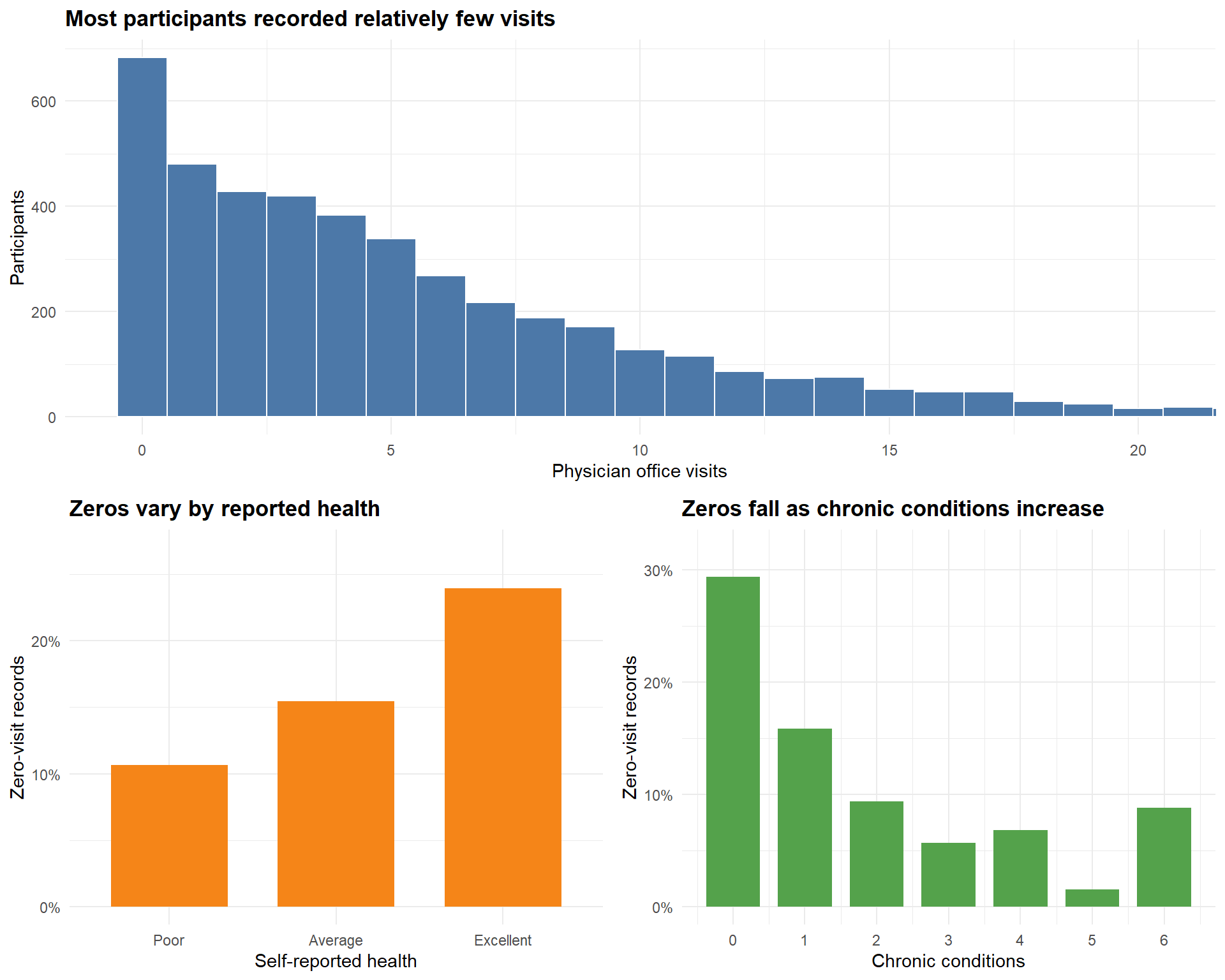
The descriptive pattern is clearest for chronic conditions. About 29% of people with no chronic conditions recorded zero visits, compared with 9% of those with two conditions and 6% of those with three. The final bars are based on smaller groups, so the variation there should be interpreted with caution.
Self-reported health shows a less linear pattern. The zero proportion is highest for people reporting excellent health (24%), followed by average health (15%) and poor health (11%). These are unadjusted comparisons: age, sex, marital status, and chronic conditions differ between the groups. We therefore cannot read the bars as isolated health-status effects, still less as evidence that any particular zero is structural.
What the plots do establish is heterogeneity: the probability of a zero changes with observed patient characteristics, which makes a separate zero process plausible enough to investigate.
3.2.2 Adjusted Associations with an Observed Zero
Collapsing the outcome to zero versus one or more visits allows an adjusted analysis of the observed zero pattern. For this end, using a simple logistic regression will give us a relatively straightforward way to estimate the associations between predictors and the likelihood of recording no visits.
In applied work, I would use this step to start a conversation with domain experts. A coefficient can show that a group has more or fewer zero records after adjustment, but it cannot tell us whether those zeros arise from good health, poor access, avoidance, eligibility rules, or an omitted variable.
Show logistic model code
# Create binary indicator: 1 = zero visits, 0 = any visits
medcare$no_visits <- ifelse(medcare$ofp == 0, 1, 0)

# Fit logistic regression
logistic_model <- glm(
  no_visits ~ healthpoor + healthexcellent + numchron + age + male + married,
  data = medcare,
  family = binomial()
)

logistic_table <- model_parameters(
  logistic_model,
  exponentiate = TRUE
) |>
  filter(Parameter != "(Intercept)") |>
  transmute(
    Predictor = recode(
      Parameter,
      healthpoor = "Poor vs average health",
      healthexcellent = "Excellent vs average health",
      numchron = "Chronic conditions (per condition)",
      age = "Age (per decade)",
      male = "Male vs female",
      married = "Married vs not married"
    ),
    `Odds ratio` = sprintf("%.2f", Coefficient),
    `95% CI` = sprintf("%.2f–%.2f", CI_low, CI_high),
    `p-value` = format.pval(p, digits = 2, eps = 0.001)
  )

knitr::kable(logistic_table, align = c("l", "r", "c", "r"))| Predictor | Odds ratio | 95% CI | p-value |
|---|---|---|---|
| Poor vs average health | 1.22 | 0.89–1.65 | 0.204 |
| Excellent vs average health | 1.24 | 0.94–1.62 | 0.129 |
| Chronic conditions (per condition) | 0.58 | 0.53–0.63 | <0.001 |
| Age (per decade) | 0.89 | 0.77–1.02 | 0.092 |
| Male vs female | 1.70 | 1.42–2.04 | <0.001 |
| Married vs not married | 0.64 | 0.53–0.78 | <0.001 |
Table 2 shows us the modelling results. We see that each additional chronic condition is associated with 42% lower odds of recording zero visits (odds ratio 0.58, 95% CI 0.53–0.63). Men have 70% higher odds of a zero than women, while married participants have 36% lower odds than those who are not married. Remember that these estimates describe associations conditional on the other variables, but do not establish causal effects.
The health-status coefficients point towards higher adjusted odds of a zero for both poor and excellent health, but the confidence intervals include 1. The data therefore do not support a clear adjusted health-status association in this specification. Likewise, the age estimate suggests that older cohorts have slightly lower odds of a zero, but its confidence interval also includes 1.
This difference between the descriptive plot and the adjusted model is useful: the plot compares health groups as observed, whilst the regression compares people with the same included covariates. Together with the descriptive plots, this model shows that zero outcomes have structure worth modelling and that their interpretation depends on the adjustment set.
3.3 Poisson Baseline
The standard starting point for count data is a Poisson regression. Even when we expect it to fail, this model provides a useful baseline:
- What relationships would a one-process count model estimate?
- How badly does the variance assumption break?
- How many zeros would this simpler model expect?
For this application, the important Poisson assumptions are:
- Conditional distribution: Given the predictors, each person’s count follows a Poisson distribution.
- Conditional equidispersion: The conditional variance equals the conditional mean, \[\text{Var}(Y_i \mid X_i) = E(Y_i \mid X_i)\]
- Independent records: Participants are independent after conditioning on the modelled predictors.
- Comparable exposure: Each count covers the same observation window; otherwise the model needs an exposure offset.
We will first interpret the conditional-mean estimates, then check whether the Poisson variance and zero probabilities fit the data. Unlike the logistic model, which asked whether a person recorded no visits, the Poisson model uses the entire count and asks how the average number of visits changes with the predictors. It therefore provides a baseline model for the count process.
Show Poisson model code
# Fit Poisson model
count_formula <- ofp ~ healthpoor + healthexcellent + numchron +
  age + male + married

poisson_model <- glm(
  count_formula,
  data = medcare,
  family = poisson()
)

poisson_table <- model_parameters(
  poisson_model,
  exponentiate = TRUE
) |>
  filter(Parameter != "(Intercept)") |>
  transmute(
    Predictor = recode(
      Parameter,
      healthpoor = "Poor vs average health",
      healthexcellent = "Excellent vs average health",
      numchron = "Chronic conditions (per condition)",
      age = "Age (per decade)",
      male = "Male vs female",
      married = "Married vs not married"
    ),
    `Rate ratio` = sprintf("%.2f", Coefficient),
    `95% CI` = sprintf("%.2f–%.2f", CI_low, CI_high),
    `p-value` = format.pval(p, digits = 2, eps = 0.001)
  )

knitr::kable(poisson_table, align = c("l", "r", "c", "r"))| Predictor | Rate ratio | 95% CI | p-value |
|---|---|---|---|
| Poor vs average health | 1.29 | 1.25–1.33 | <0.001 |
| Excellent vs average health | 0.70 | 0.66–0.75 | <0.001 |
| Chronic conditions (per condition) | 1.18 | 1.17–1.19 | <0.001 |
| Age (per decade) | 0.95 | 0.93–0.97 | <0.001 |
| Male vs female | 0.90 | 0.88–0.93 | <0.001 |
| Married vs not married | 1.00 | 0.97–1.03 | 0.93 |
Table 3 presents the results of the Poisson regression. As a quick reminder, a Poisson rate ratio describes a proportional difference in the expected count: the average number of visits predicted for people with the same included characteristics.
Here, under the Poisson mean model, poor health is associated with a 29% higher expected visit count than average health, while excellent health is associated with a 30% lower count. Each additional chronic condition is associated with an 18% increase. Men have an expected count about 10% lower than women, and a decade of age is associated with a 5% reduction. The estimate for marital status is essentially null.
3.4 Where the Poisson Model Fails
Now that we have our fitted mean structure, the next step is to check whether the Poisson distribution adequately describes the conditional variation. The Pearson residuals provide a direct assessment of equidispersion after adjustment for the predictors.
Show overdispersion diagnostic code
overdispersion_check <- check_overdispersion(poisson_model)

overdispersion_table <- tibble::tibble(
  Metric = c(
    "Pearson chi-squared",
    "Residual degrees of freedom",
    "Dispersion ratio",
    "p-value"
  ),
  Value = c(
    format(
      round(overdispersion_check$chisq_statistic),
      big.mark = ","
    ),
    format(
      overdispersion_check$residual_df,
      big.mark = ","
    ),
    sprintf("%.2f", overdispersion_check$dispersion_ratio),
    format.pval(overdispersion_check$p_value, digits = 2, eps = 0.001)
  )
)

knitr::kable(overdispersion_table)| Metric | Value |
|---|---|
| Pearson chi-squared | 31,664 |
| Residual degrees of freedom | 4,399 |
| Dispersion ratio | 7.20 |
| p-value | <0.001 |
TipWhat is overdispersion?
Remember that overdispersion occurs when the conditional variance of the observed counts exceeds the variance allowed by the model. For a Poisson model, the conditional mean and variance must be equal. A dispersion ratio substantially above 1 indicates that this assumption is inadequate.
The dispersion ratio is 7.20, well above the value of 1 expected under a Poisson model. The observed visit counts therefore vary much more than the model permits under the Poisson assumption. This overdispersion makes the model-based standard errors too small and the corresponding confidence intervals and p-values too optimistic. The rate ratios still summarize the fitted mean structure, but this means that the Poisson model does not provide reliable inference for these data.
Overdispersion identifies the Poisson model as inadequate but does not identify the source of the extra variation. The next one-process candidate is therefore negative binomial regression, which relaxes the equidispersion assumption without introducing a latent extra-zero group.
3.5 Negative-Binomial Fit and Zero-Frequency Comparison
The negative binomial baseline retains the count_formula used above, so it makes the same conditional comparisons as the Poisson model. Its nbinom2 variance, \(\mu_i + \mu_i^2/\phi\), allows variation to increase faster than the mean.
nb_model <- glmmTMB(
  count_formula,
  data = medcare,
  family = nbinom2()
)
After fitting this model, the dispersion parameter is \(\hat{\phi} =\) 1.13. This finite value allows substantially more conditional variation than Poisson; remember that the Poisson limit would require \(\phi \to \infty\). The model still treats every participant as arising from one count-generating process.
Zero prediction isolates one important consequence of the different variance assumptions. For participant \(i\), the fitted Poisson probability of zero is
\[P(Y_i = 0) = e^{-\hat{\lambda}_i}\]
whereas the fitted NB2 probability is
\[P(Y_i = 0) = \left(\frac{\hat{\phi}}{\hat{\phi}+\hat{\mu}_i}\right)^{\hat{\phi}}.\]
Summing the person-specific probabilities gives the expected number of zero-visit records under each model.
Show zero-frequency comparison code
# Observed zeros
observed_zeros <- sum(medcare$ofp == 0)

# Predicted zeros from Poisson model
poisson_pred <- predict(poisson_model, type = "response")
poisson_zero_prob <- exp(-poisson_pred)  # P(Y=0) for Poisson
expected_zeros_poisson <- sum(poisson_zero_prob)

# Predicted zeros from negative binomial model
nb_mean <- predict(nb_model, type = "conditional")
nb_dispersion <- predict(nb_model, type = "disp")
nb_zero_prob <- dnbinom(0, mu = nb_mean, size = nb_dispersion)
expected_zeros_nb <- sum(nb_zero_prob)

zero_comparison <- tibble::tibble(
  Model = c("Poisson", "Negative binomial (NB2)"),
  `Expected zeros` = round(c(
    expected_zeros_poisson,
    expected_zeros_nb
  )),
  `Observed minus expected` = observed_zeros - `Expected zeros`,
  `Expected / observed` = sprintf(
    "%.1f%%",
    100 * `Expected zeros` / observed_zeros
  )
)

knitr::kable(
  zero_comparison,
  align = c("l", "r", "r", "r")
)| Model | Expected zeros | Observed minus expected | Expected / observed |
|---|---|---|---|
| Poisson | 37 | 646 | 5.4% |
| Negative binomial (NB2) | 623 | 60 | 91.2% |
The fitted Poisson model expects approximately 37 zero-visit records, only 5.4% of the 683 observed. NB2 expects approximately 623, or 91.2% of the observed number. Allowing extra variation within one count process therefore explains most of what initially looked like a zero surplus.
The remaining shortfall is about 60 zero records. That discrepancy keeps a separate extra-zero process under consideration, but it does not prove that such a process exists. Misspecification of the conditional mean, other forms of heterogeneity, or a different count distribution could also affect zero prediction.
The baseline analysis has therefore narrowed rather than settled the question. Poisson is too restrictive, while NB2 captures most of the dispersion and zero frequency without a latent class. Section 4 introduces the extra-zero mechanism so that its additional structure can be compared with this stronger one-process benchmark.
4 How Zero-Inflated Models Work
4.1 A Latent Two-Process Model
After setting our benchmark analysis, we are finally ready to introduce the zero-inflated model. Unlike the negative binomial baseline, which keeps every participant in one count process, a zero-inflated model allows either of two states to generate each observed count. For participant \(i\), we introduce \(S_i\) as a binary indicator of that state.
- \(S_i=1\) means the extra-zero state is active. In this state, the recorded number of visits must be zero.
- \(S_i=0\) means the count-generating state is active. This state can produce either zero visits or a positive number of visits.
The state is latent because it is not recorded in the data. When a participant has zero visits, we do not know which state generated that zero. The idea is to model the probability that an individual patient will fall under each state.
This probability may vary across patient profiles. Let \(Z_i\) contain the predictors used for this part of the model, and let \(\pi_i\) be the resulting probability that participant \(i\) is in the extra-zero state. We write
\[ \begin{aligned} S_i \mid Z_i &\sim \operatorname{Bernoulli}(\pi_i), \\ P(S_i=1\mid Z_i) &= \pi_i. \end{aligned} \]
In other words, \(S_i\) takes the value 1 with probability \(\pi_i\), based on the participant’s zero-inflation predictors \(Z_i\).
Now let \(Y_i\) be the observed number of visits and let \(X_i\) contain the predictors used for the count component. The outcome model formalizes the two states described above:
\[ \begin{aligned} Y_i \mid S_i=1 &\equiv 0, \\ Y_i \mid S_i=0,X_i &\sim f_c(\,\cdot\,;\mu_i,\psi). \end{aligned} \]
When the extra-zero state is active, by definition the number of visits must be zero. In the count-generating state, visits follow \(f_c\), a count distribution with mean \(\mu_i\). The placeholder \(\psi\) represents a family-specific dispersion parameter when one is required: it is absent for Poisson and equals \(\phi\) for the NB2 model used later.
In essence, and forgetting about notation for a moment, the central idea is that the extra-zero state always produces zero, whereas the count-generating state can produce either zero or a positive count. Figure 4 illustrates this two-stage process.
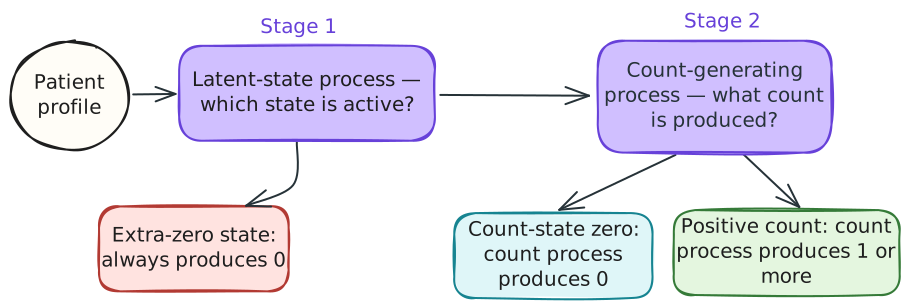
For the Medicare data, the two components therefore ask different questions. The zero-inflation component asks which patient profiles receive a higher probability of the extra-zero state. The count component asks how expected visits change within the count-generating state.
4.2 Mixture Probabilities and Likelihood
Zeros are ambiguous because either latent state can produce them. Positive counts are not: they can come only from the count-generating state. This asymmetry gives the model information about both components. It estimates them jointly from all observations rather than classifying the zeros first and then fitting separate regressions.
Let \(f_c(k;\mu_i,\psi)\) denote the probability that the count component assigns to the value \(k\). The possible routes are:
- If \(y_i=0\), the observation may come directly from the extra-zero state, with probability \(\pi_i\), or from the count-generating state producing zero, with probability \((1-\pi_i)f_c(0;\mu_i,\psi)\).
- If \(y_i>0\), the observation has one possible route: the count-generating state, with probability \((1-\pi_i)f_c(y_i;\mu_i,\psi)\).
The likelihood contribution \(L_i\) is the probability that the model assigns to the outcome observed for participant \(i\). The two cases above give
\[ L_i(\pi_i,\mu_i,\psi) = \begin{cases} \pi_i+(1-\pi_i)f_c(0;\mu_i,\psi), & y_i=0, \\ (1-\pi_i)f_c(y_i;\mu_i,\psi), & y_i>0. \end{cases} \]
In each case, \(L_i\) is the probability that the model assigns to participant \(i\)’s observed outcome. For a zero, the contribution adds the probabilities of both routes instead of choosing one. Across the sample, these contributions form a single objective for estimating the count, zero-inflation, and dispersion parameters together.
CautionThe full likelihood
Multiplying the contributions from all \(n\) participants gives the full likelihood. The coefficient vectors \(\beta\) and \(\gamma\) govern the count and zero-inflation components, respectively:
\[ L(\beta,\gamma,\psi) = \prod_{i=1}^{n} L_i\bigl(\pi_i(\gamma),\mu_i(\beta),\psi\bigr). \]
Maximizing this product estimates the count, zero-inflation, and dispersion parameters jointly.
Joint estimation also explains why the preliminary logistic regression in Table 2 does not represent the fitted zero-inflation component by itself. The preliminary regression models the observed event \(Y_i=0\), regardless of which state produced the zero. The fitted zero-inflation component models the latent event \(S_i=1\). These are different outcomes: the probability of an observed zero includes both routes, whereas \(\pi_i\) is the model probability of the extra-zero state.
Because the state remains unobserved, a zero raises the practical question: given that we observed a zero, what is the probability that it came from the extra-zero state rather than from the count-generating state? The posterior probability below answers that question. Bayes’ rule first expresses it in terms of model probabilities:
\[ \begin{aligned} P(S_i=1\mid Y_i=0,X_i,Z_i) &= \frac{ P(Y_i=0\mid S_i=1)P(S_i=1\mid Z_i) }{ P(Y_i=0\mid X_i,Z_i) } \\ &= \frac{ 1\times\pi_i }{ \pi_i+(1-\pi_i)f_c(0;\mu_i,\psi) }. \end{aligned} \]
The first numerator term equals one because the extra-zero state always produces zero. The prior model probability of that state is \(\pi_i\) by definition of the zero-inflation component. The denominator contains both routes to an observed zero: the extra-zero route and a zero from the count-generating state. For a positive count, the posterior probability of the extra-zero state is zero because that state cannot produce a positive value.
For a concrete example with a Poisson count component, suppose the model assigns observations with a particular covariate profile an extra-zero probability \(\pi_i=0.15\) and a count-component mean \(\lambda_i=3.2\).
- Within the count-generating state, the probability of zero visits is \(e^{-3.2}=0.041\), or 4.1%.
- Combining both routes gives an overall zero probability of \(0.15+0.85(0.041)=0.185\), or 18.5%.
- If an observation with this profile equals zero, the posterior probability of the extra-zero state is \(0.15/0.185\approx0.81\), or 81%.
The key idea is that this posterior probability therefore updates uncertainty about the latent state. Because the count component considers zero unlikely for this profile, observing zero shifts much of the model’s probability toward the extra-zero state! This soft assignment helps estimate the two components jointly.
4.3 Mixture Mean and Variance
Once the model has estimated the extra-zero probability and the behaviour of the count-generating state, we can ask what it predicts for observed visits. Here, \(\mu_i\) is the mean of the chosen count distribution for participant \(i\) within the count-generating state. Let \(V_c(\mu_i)\) denote the corresponding variance:
\[ \begin{aligned} E(Y_i\mid S_i=0,X_i) &= \mu_i, \\ \operatorname{Var}(Y_i\mid S_i=0,X_i) &= V_c(\mu_i). \end{aligned} \]
In a single-process count model, \(\mu_i\) would also be the expected observed count. In a zero-inflated model, however, the model assigns some probability to an always-zero state. We must average over both states to obtain expected observed visits.
The extra-zero state contributes zero with probability \(\pi_i\), while the count-generating state contributes an average of \(\mu_i\) with probability \(1-\pi_i\). Therefore,
\[ E(Y_i\mid X_i,Z_i) =\pi_i(0)+(1-\pi_i)\mu_i =(1-\pi_i)\mu_i. \]
This conditional mixture mean is conditional on the observed predictors \(X_i\) and \(Z_i\), but averages over the unobserved state \(S_i\). It is the quantity we need when comparing expected visits across patient profiles. Reporting \(\mu_i\) instead would describe only the count-generating state and would overstate expected observed visits whenever \(\pi_i>0\).
The mean alone does not tell us how observations are distributed around that average. Two fitted distributions can predict the same expected number of visits while assigning very different probabilities to zero, moderate, and high counts. The mixture variance summarizes this spread, so it helps us judge whether the fitted distribution represents the observed pattern of visits.
CautionDeriving the mixture variance
The law of total variance separates variation within the latent states from variation between their conditional means.
Within-state variation is the variation that remains after fixing the latent state. The extra-zero state contributes no variance because it always produces zero. The count-generating state contributes \(V_c(\mu_i)\) and occurs with probability \(1-\pi_i\). Therefore,
\[ \begin{gathered} E\!\left[ \operatorname{Var}(Y_i\mid S_i,X_i,Z_i) \right] \\ =\pi_i(0)+(1-\pi_i)V_c(\mu_i) \\ =(1-\pi_i)V_c(\mu_i). \end{gathered} \]
Between-state variation arises because the states have different means: zero in the extra-zero state and \(\mu_i\) in the count-generating state. The state-specific mean can be written as \(\mu_i(1-S_i)\). Because \(S_i\) is Bernoulli with probability \(\pi_i\),
\[ \begin{gathered} \operatorname{Var}\!\left[ E(Y_i\mid S_i,X_i,Z_i) \right] \\ =\mu_i^2\operatorname{Var}(1-S_i) \\ =\pi_i(1-\pi_i)\mu_i^2. \end{gathered} \]
Adding the within-state and between-state contributions gives the mixture variance:
\[ \operatorname{Var}(Y_i\mid X_i,Z_i) = \underbrace{(1-\pi_i)V_c(\mu_i)}_{\text{within-state variation}} + \underbrace{\pi_i(1-\pi_i)\mu_i^2}_{\text{between-state variation}}. \]
The count distribution determines \(V_c(\mu_i)\). A Poisson count state has \(V_c(\mu_i)=\mu_i\), giving a zero-inflated Poisson (ZIP) model. An NB2 count state has \(V_c(\mu_i)=\mu_i+\mu_i^2/\phi\), giving a zero-inflated negative-binomial (ZINB) model. The resulting mixture variances are shown below.
| Model | Count-state zero probability \(f_c(0)\) | Count-state variance \(V_c(\mu_i)\) | Conditional mixture variance |
|---|---|---|---|
| ZIP | \(e^{-\mu_i}\) | \(\mu_i\) | \((1-\pi_i)\mu_i+\pi_i(1-\pi_i)\mu_i^2\) |
| ZINB (NB2) | \(\left(\dfrac{\phi}{\phi+\mu_i}\right)^\phi\) | \(\mu_i+\dfrac{\mu_i^2}{\phi}\) | \((1-\pi_i)\left(\mu_i+\dfrac{\mu_i^2}{\phi}\right)+\pi_i(1-\pi_i)\mu_i^2\) |
Both models have conditional mixture mean \((1-\pi_i)\mu_i\). Their difference lies in the spread around that mean. ZIP uses a Poisson count state, whereas ZINB adds the term \(\mu_i^2/\phi\) and therefore allows overdispersion within the count-generating state. As \(\phi\to\infty\), that additional variation disappears and the ZINB expressions approach their ZIP counterparts.
For the Medicare case study, the mean identity tells us how to calculate expected observed visits, while the variance distinguishes what each count distribution can represent. The next section connects \(\pi_i\) and \(\mu_i\) to predictors and asks how changes in either component affect the overall mean.
4.4 Regression and Overall Effects
We have seen that the overall mean depends on both the count-state mean \(\mu_i\) and the extra-zero probability \(\pi_i\). The next question is then: how does a predictor change that mean?
In a zero-inflated model, a predictor may change expected visits within the count-generating state, the probability of the extra-zero state, or both. Its component coefficient therefore need not describe its association with observed visits.
Let \(X_i\) contain the count-component predictors and let \(\beta\) contain their coefficients. Let \(Z_i\) contain the zero-inflation predictors and let \(\gamma\) contain their coefficients. In glmmTMB, the zero-inflation component always uses a logit link. The count-component link is more flexible: the log link is the default for the Poisson and NB2 distributions used here, as it is for most count distributions available in glmmTMB, but it can be changed. The models in this tutorial therefore use
\[ \begin{aligned} \log(\mu_i) &= X_i\beta, \\ \operatorname{logit}(\pi_i) &= Z_i\gamma. \end{aligned} \]
The log link keeps \(\mu_i\) positive, while the logit link keeps \(\pi_i\) between zero and one. A predictor may appear in either equation or in both.
Count component: For a predictor \(x_j\) in \(X_i\), \(e^{\beta_j}\) is the rate ratio for a one-unit increase in \(x_j\), holding the other count-component predictors fixed. It describes how \(\mu_i\) changes within the count-generating state.
Zero-inflation component: For a predictor \(x_j\) in \(Z_i\), \(e^{\gamma_j}\) is the odds ratio for the extra-zero state. A value above one means that a one-unit increase in \(x_j\) raises the modelled odds of that state, holding the other zero-inflation predictors fixed.
Neither coefficient alone answers the practical question: how do expected observed visits change? That quantity still requires both components, which as we have seen in the previous section, is given by:
\[ m_i =E(Y_i\mid X_i,Z_i) =(1-\pi_i)\mu_i. \]
In essence, the two pathways can reinforce or offset one another. Suppose a one-unit increase in a predictor raises \(\mu_i\) from 4 to 5 but also raises \(\pi_i\) from 0.10 to 0.30. The count-state mean increases by 25%, yet the overall mean falls slightly, from \((1-0.10)4=3.6\) to \((1-0.30)5=3.5\). The higher extra-zero probability more than offsets the higher count-state mean. If \(\mu_i\) rises while \(\pi_i\) falls, the two pathways instead reinforce one another.
CautionCombining both pathways
For the additive linear predictors used here, suppose \(x_j\) appears in both components. A one-unit increase gives the overall expected-count ratio
\[ \frac{m_i(x_j+1)}{m_i(x_j)} = \underbrace{e^{\beta_j}}_{\text{count-state change}} \underbrace{ \frac{1-\pi_i(x_j+1)}{1-\pi_i(x_j)} }_{\text{count-state probability change}}. \]
The first factor is the change in the count-state mean. The second is the change in the probability of being in the count-generating state. If \(x_j\) appears only in the count component, the second factor equals one. If it appears only in the zero-inflation component, the first factor equals one.
Unlike the count-state factor \(e^{\beta_j}\), the second factor depends on the starting value of \(\pi_i\). The combined ratio can therefore vary across patient profiles.
Because the pathways can reinforce or offset one another, component coefficient tables do not show how expected observed visits change. Section 5 therefore uses response-scale predictions of \(m_i\) rather than stopping at rate ratios and odds ratios. Before fitting those models, however, we must decide which predictors belong in each component.
4.5 Choosing Predictors
As we have seen in the previous section, placing a variable in one formula but not the other restricts which part of the outcome distribution it may change, and as such is an important choice to make.
The two components pose different questions:
- Which variables describe visit intensity within the count-generating state?
- Which variables plausibly describe the probability of the extra-zero state?
The count component retains the baseline adjustment set used in the Poisson analysis:
ofp ~ healthpoor + healthexcellent + numchron + age + male + marriedThese predictors represent health need and demographic differences that may be associated with visit rates. Their inclusion defines the conditional comparison; it does not turn the resulting coefficients into causal effects.
Two available variables are deliberately left out. hosp counts hospital stays during the same observation period as the office visits, so treating it as a prior predictor would blur the temporal ordering between two concurrent measures of healthcare use. school records years of education and could reasonably enter as a socioeconomic covariate. We leave it out to keep the teaching specification focused. This count formula is a starting point, and a fuller analysis would compare other substantively plausible alternatives.
Ideally, the zero-inflation formula would include direct measures of why someone cannot or does not enter the visit-generating process, such as eligibility restrictions, insurance coverage, or geographic access. The medcare data unfortunately contain no such measures. Its health and demographic variables can describe systematic differences in the estimated extra-zero probability, but they cannot identify the mechanism behind those differences.
For the initial ZIP and ZINB comparison, the zero-inflation component will use the more compact formula:
~ numchron + male + marriedChronic conditions, sex, and marital status showed the clearest adjusted associations with an observed zero in Table 2. That result provides an empirical starting point, but it’s not a direct measurement of extra-zero membership: as established in Section 4.3, observed zeros combine both possible routes to zero.
These three predictors therefore enter both components initially, allowing each to be associated with visit intensity and with the estimated extra-zero probability. Including or excluding a predictor imposes a substantive restriction, and the available variables provide only indirect support for either choice. In the next section we will therefore also compare some alternative zero-inflation specifications.
5 Fitting, Checking, and Interpreting the Models
The predictor-selection discussion showed that predictor placement changes what a zero-inflated model represents: the count formula governs \(\mu_i\), while the zero formula governs \(\pi_i\). Model comparison must therefore distinguish the count distribution from the presence and specification of the extra-zero component. We will address three decisions in order:
- Does the count component require NB2 rather than Poisson variation?
- After allowing NB2 variation, does the model benefit from any extra-zero component?
- If it does, should the extra-zero probability be constant or vary with patient characteristics?
Each question requires a matched contrast. Poisson and NB2 use the same count formula and no zero component. Ordinary NB2 and intercept-only ZINB use the same count formula and count family; ziformula = ~ 1 adds one constant extra-zero probability rather than allowing it to vary across records. The intercept-only and covariate-dependent ZINBs then hold the NB2 count process fixed while changing only the zero formula.
ZIP remains useful for a different contrast. Comparing ZIP with the compact ZINB holds both formulas fixed and asks whether the count component still needs NB2 variation inside a zero-inflated model. ZIP can therefore show why adding an extra-zero component does not repair an inadequate Poisson count distribution. Comparing ZIP directly with ordinary NB2 would change both the count family and the zero formula, so it would not isolate evidence for an extra-zero component.
5.1 Fit Matched Candidate Specifications
For the sake of simplicity and exposition, every specification considered here uses the same count formula:
ofp ~ healthpoor + healthexcellent + numchron + age + male + marriedThe Poisson baseline uses the Poisson family with no zero component, while the negative-binomial baseline uses NB2 with no zero component. This subsection adds only the candidates needed for the first comparisons:
- Compact ZIP: Poisson count family with
~ numchron + male + marriedas its zero formula. - Intercept-only ZINB: NB2 count family with
~ 1as its zero formula. - Compact ZINB: NB2 count family with
~ numchron + male + marriedas its zero formula.
Additional zero-component formulas are deferred until their rationale is introduced.
1compact_zi_formula <- ~ numchron + male + married

# Compact zero-inflated Poisson model
zip_model <- glmmTMB(
  count_formula,
2  ziformula = compact_zi_formula,
  data = medcare,
  family = poisson()
)

# Intercept-only zero-inflated NB2 model
zinb_intercept_model <- glmmTMB(
  count_formula,
3  ziformula = ~ 1,
  data = medcare,
  family = nbinom2()
)

zinb_compact_model <- glmmTMB(
  count_formula,
  ziformula = compact_zi_formula,
  data = medcare,
4  family = nbinom2()
)- 1
- The compact zero formula carries forward the clearest adjusted associations with observed zeros from Table 2.
- 2
- Compact ZIP and compact ZINB use the same count and zero formulas, so their contrast changes only the count distribution.
- 3
-
With
nbinom2(),ziformula = ~ 1assigns every record the same fitted probability of the latent extra-zero state. The NB2 count mean can still vary with the predictors incount_formula. - 4
-
Pairing a covariate-dependent
ziformulawithnbinom2()lets the extra-zero probability vary across patient characteristics while retaining NB2 variation in the count process.
We compare these specifications in matched pairs because each pair isolates one modelling decision: the count family, the addition of a constant extra-zero probability, or whether that probability varies with patient characteristics.
It’s important to keep in mind that the resulting fit statistics provide relative evidence among the specifications, but they neither identify a distinct extra-zero population nor replace distributional diagnostics, which are still needed to assess whether the chosen count distribution adequately represents the data.
5.2 Separate Count-Family and Zero-Component Evidence
The fitted specifications now let us separate the three decisions posed at the start of this section. We first compare Poisson with NB2, using both the ordinary and zero-inflated versions, to choose the count family. We then return to the ordinary NB2 baseline and add the simplest possible extra-zero component before asking whether that component should vary across patient characteristics.
Both AIC and BIC ask whether an improvement in likelihood is worth the additional parameters. Lower values favour a specification, but only differences among models fitted to the same observations with compatible likelihoods are meaningful. AIC emphasises expected predictive accuracy, whereas BIC is more reluctant to add parameters at this sample size, so comparing them shows how sensitive the result is to the penalty for complexity. These scores can rank the candidates considered here; the residual checks later will show whether the leading models are actually able to reproduce the data.
How large do these differences need to be? There is no universal pass-or-fail cutoff. Values that are close together indicate little separation between two specifications, whereas gaps of hundreds or thousands show a clear preference for the model with the lower value.
Show model-comparison code
models <- list(
  Poisson = poisson_model,
  NB2 = nb_model,
  `Compact ZIP` = zip_model,
  `Intercept-only ZINB` = zinb_intercept_model,
  `Compact ZINB` = zinb_compact_model
)

comparison_table <- tibble::tibble(
  Model = names(models),
  AIC = vapply(models, AIC, numeric(1)),
  BIC = vapply(models, BIC, numeric(1)),
  RMSE = vapply(
    models,
    function(model) {
      predictions <- predict(model, type = "response")
      sqrt(mean((medcare$ofp - predictions)^2))
    },
    numeric(1)
  )
) |>
  mutate(
    across(c(AIC, BIC), ~ round(.x, 1)),
    RMSE = round(RMSE, 3)
  )

knitr::kable(comparison_table, align = c("l", "r", "r", "r"))| Model | AIC | BIC | RMSE |
|---|---|---|---|
| Poisson | 37093.4 | 37138.1 | 6.505 |
| NB2 | 24576.1 | 24627.2 | 6.529 |
| Compact ZIP | 33115.3 | 33185.6 | 6.488 |
| Intercept-only ZINB | 24574.4 | 24631.9 | 6.525 |
| Compact ZINB | 24458.0 | 24534.7 | 6.496 |
We start with the count family. Moving from Poisson to NB2 lowers AIC from 37093.4 to 24576.1 when neither model has an extra-zero component. Holding the compact zero formula fixed leads to the same conclusion: moving from ZIP to compact ZINB lowers AIC from 33115.3 to 24458.0. BIC tells the same story in both comparisons. These gaps leave little doubt that Poisson variation is too restrictive here, whether or not the model includes an extra-zero component.
The next question is whether NB2 needs an extra-zero component at all. The cleanest starting point is intercept-only ZINB: it keeps the NB2 count process unchanged and assigns every participant the same extra-zero probability. Compared with ordinary NB2, its AIC is only 1.7 points lower, while its BIC is 4.7 points higher. The small AIC gap and the reversal under BIC suggest that a constant extra-zero probability adds little to the ordinary NB2 model.
What changes when the extra-zero probability can vary between participants? Relative to intercept-only ZINB, the compact ZINB lowers AIC by 116.4 points and BIC by 97.2 points. Both gaps are large: allowing the zero component to vary with chronic conditions, sex, and marital status improves the fitted distribution substantially. It does not, however, show that the zeros came from a separate, identifiable group of patients.
The root mean squared error (RMSE) column appears to disagree with AIC and BIC because it assesses only the predicted average. For each participant, RMSE compares the observed count with the model’s expected count, but does not consider how much probability the model assigned to that count or to other possible counts. Compact ZIP therefore achieves the lowest RMSE, 6.488, even though its AIC and BIC are much higher than those of the NB2 models.
Two models can predict similar averages while assigning very different probabilities to zeros, moderate counts, and unusually high counts. If prediction became a primary goal, repeated cross-validation should assess a score for the entire predictive distribution, such as held-out log predictive density or ranked probability score, alongside RMSE.
The comparison therefore narrows the next decision: retain NB2 variation in the count component, then ask which covariate-dependent zero formula, if any, provides a defensible working specification.
5.3 Choose the Zero-Component Specification
The preceding comparison showed that adding a constant extra-zero probability to NB2 changes fit very little, whereas allowing that probability to vary across participants produces a much larger improvement. That result leaves an important specification question: which participant characteristics should be allowed to change the extra-zero probability?
Starting from the intercept-only ZINB, we compare three ways of allowing that probability to vary:
- The excellent-health specification represents a narrow health-need explanation;
- The compact specification carries forward the strongest adjusted associations with an observed zero in these data;
- The shared-adjustment specification allows every count predictor to have a separate zero-component association.
All four models retain the same NB2 count family and count formula, so the comparison concerns only the zero-component specification. This small candidate set tests whether the compact model’s improvement depends on its particular formula and whether the broader specification earns its additional complexity.
Show ZINB specification-comparison code
zinb_spec_models <- list(
  `Intercept-only` = zinb_intercept_model,
  `Excellent-health only` = glmmTMB(
    count_formula,
    ziformula = ~ healthexcellent,
    data = medcare,
    family = nbinom2()
  ),
  Compact = zinb_compact_model,
  `Shared adjustment set` = glmmTMB(
    count_formula,
    ziformula = ~ healthpoor + healthexcellent + numchron +
      age + male + married,
    data = medcare,
    family = nbinom2()
  )
)

zinb_model <- zinb_spec_models[["Compact"]]

zinb_spec_table <- tibble::tibble(
  Specification = names(zinb_spec_models),
  `Zero-inflation formula` = c(
    "~ 1",
    "~ healthexcellent",
    sub("^~", "~ ", format(compact_zi_formula)),
    "~ healthpoor + healthexcellent + numchron + age + male + married"
  ),
  `Substantive restriction` = c(
    "Keeps the extra-zero probability constant across participants.",
    "Allows an excellent-health difference, but none by the other predictors; average and poor health share the same fitted probability.",
    "Allows differences by chronic-condition count, sex, and marital status; excludes age and additional self-rated-health differences.",
    "Allows each count predictor its own zero-component association; imposes the fewest restrictions at the cost of three additional coefficients."
  ),
  AIC = vapply(zinb_spec_models, AIC, numeric(1)),
  BIC = vapply(zinb_spec_models, BIC, numeric(1))
) |>
  mutate(
    across(c(AIC, BIC), ~ round(.x, 1))
  ) |>
  arrange(AIC)

knitr::kable(zinb_spec_table, align = c("l", "l", "l", "r", "r"))| Specification | Zero-inflation formula | Substantive restriction | AIC | BIC |
|---|---|---|---|---|
| Shared adjustment set | ~ healthpoor + healthexcellent + numchron + age + male + married | Allows each count predictor its own zero-component association; imposes the fewest restrictions at the cost of three additional coefficients. | 24457.8 | 24553.6 |
| Compact | ~ numchron + male + married | Allows differences by chronic-condition count, sex, and marital status; excludes age and additional self-rated-health differences. | 24458.0 | 24534.7 |
| Intercept-only | ~ 1 | Keeps the extra-zero probability constant across participants. | 24574.4 | 24631.9 |
| Excellent-health only | ~ healthexcellent | Allows an excellent-health difference, but none by the other predictors; average and poor health share the same fitted probability. | 24576.0 | 24639.9 |
The four zero formulas are not all nested, so no single likelihood-ratio test can compare all of them. We therefore use the information-criterion framework introduced above: AIC for relative in-sample comparison and BIC as a stronger parsimony check.
The results give us little reason to carry forward the intercept-only or excellent-health-only models. As the preceding comparison showed, the intercept-only model receives little support beyond ordinary NB2. Allowing the extra-zero probability to vary only with excellent health does no better: its AIC is 24576.0 and its BIC is 24639.9, both higher than the intercept-only model’s values of 24574.4 and 24631.9. A single excellent-health indicator is therefore too narrow to reproduce the improvement seen with the compact formula.
That leaves the compact and shared-adjustment specifications. The shared-adjustment model lowers AIC by only 0.2 points, from 24458.0 to 24457.8, but raises BIC by 18.9 points. I therefore keep the compact formula: the three extra coefficients in the shared-adjustment model make almost no difference to AIC and incur a much larger BIC penalty.
The compact formula was chosen partly after examining adjusted associations with an observed zero in this same dataset, and remains a provisional teaching specification.
Given the results, for the rest of the article, we carry forward ~ numchron + male + married as the provisional compact ZINB working specification. The confidence intervals and p-values reported later treat this formula as if it had been fixed before the analysis. They do not account for the predictor-selection step.
Finally, before relying on these comparisons, it’s good practice to check whether each candidate produced a numerically trustworthy solution. A successful optimizer termination, a positive-definite Hessian, and finite standard errors indicate that the software found a well-defined optimum. Large zero-component coefficients can instead signal a nearly flat likelihood in which the extra-zero probability approaches zero or one.
NoteChecking for estimation stability
The code below applies the same checks to every glmmTMB candidate used in the information-criterion comparisons. It then reports the number of flagged candidates and shows the compact ZINB as a worked example. The supplementary diagnose() call checks coefficient magnitudes, predictor scaling, and Hessian curvature. We disable its large-\(z\) screen because a precisely estimated association is not by itself an optimization failure.
Show estimation-stability checks for the fitted candidates.
candidate_glmmtmb_models <- c(
  list(
    NB2 = nb_model,
    `Compact ZIP` = zip_model
  ),
  setNames(
    zinb_spec_models,
    paste(names(zinb_spec_models), "ZINB")
  )
)

check_estimation_stability <- function(model) {
  coefficient_blocks <- summary(model)$coefficients
  standard_errors <- unlist(lapply(
    coefficient_blocks,
    function(block) {
      if (is.null(block) || nrow(block) == 0) {
        return(numeric(0))
      }
      block[, "Std. Error"]
    }
  ))
  zero_coefficients <- unname(fixef(model)$zi)

  # diagnose() prints a short message, so capture it while retaining its result.
  diagnose_message <- capture.output(
    diagnose_ok <- glmmTMB::diagnose(
      model,
      check_zstats = FALSE,
      explain = FALSE
    )
  )

  tibble::tibble(
    optimizer_ok = model$fit$convergence == 0,
    hessian_ok = isTRUE(model$sdr$pdHess),
    finite_se = length(standard_errors) > 0 &&
      all(is.finite(standard_errors)),
    extreme_zero_coefficient = length(zero_coefficients) > 0 &&
      any(abs(zero_coefficients) > 10),
    diagnose_ok = isTRUE(diagnose_ok)
  )
}

stability_checks <- dplyr::bind_rows(
  lapply(candidate_glmmtmb_models, check_estimation_stability),
  .id = "Model"
) |>
  mutate(
    all_checks_pass = optimizer_ok & hessian_ok & finite_se &
      !extreme_zero_coefficient & diagnose_ok
  )

compact_checks <- stability_checks |>
  filter(Model == "Compact ZINB")

stability_status <- bind_rows(
  tibble::tibble(
    Scope = "All comparison candidates",
    Check = "Candidates with one or more flagged checks",
    Result = sprintf(
      "%d of %d",
      sum(!stability_checks$all_checks_pass),
      nrow(stability_checks)
    )
  ),
  tibble::tibble(
    Scope = "Compact ZINB",
    Check = c(
      "Optimizer termination",
      "Positive-definite Hessian",
      "Finite standard errors",
      "Zero-component coefficient magnitude",
      "Supplementary diagnose() checks"
    ),
    Result = c(
      ifelse(compact_checks$optimizer_ok, "Passed", "Flagged"),
      ifelse(compact_checks$hessian_ok, "Passed", "Flagged"),
      ifelse(compact_checks$finite_se, "Passed", "Flagged"),
      ifelse(
        compact_checks$extreme_zero_coefficient,
        "Flagged",
        "No coefficient with |estimate| > 10"
      ),
      ifelse(compact_checks$diagnose_ok, "Passed", "Flagged")
    )
  )
)

knitr::kable(stability_status, align = c("l", "l", "l"))| Scope | Check | Result |
|---|---|---|
| All comparison candidates | Candidates with one or more flagged checks | 0 of 6 |
| Compact ZINB | Optimizer termination | Passed |
| Compact ZINB | Positive-definite Hessian | Passed |
| Compact ZINB | Finite standard errors | Passed |
| Compact ZINB | Zero-component coefficient magnitude | No coefficient with |estimate| > 10 |
| Compact ZINB | Supplementary diagnose() checks | Passed |
diagnose() is an experimental troubleshooting aid, so the explicit optimizer, Hessian, standard-error, and coefficient checks remain visible rather than being replaced by one package-generated verdict.
All six glmmTMB candidates passed these checks, including the compact ZINB shown above. Their likelihood comparisons and coefficient estimates therefore show no evident numerical warning.
5.4 Check Distributional Fit
We now examine how closely the compact ZINB reproduces the observed visit counts. DHARMa simulates outcomes from the fitted model and compares each observation with its simulated distribution. It expresses the result as a scaled residual between 0 and 1; a well-calibrated model should produce residuals that are approximately uniform across that interval.
CautionDHARMa’s scaled residuals
For participant \(i\), let \(y_i\) be the observed count and let \(y_i^{(1)}, \ldots, y_i^{(S)}\) denote \(S\) responses simulated from the conditional fitted distribution implied by the model. In this tutorial, that distribution is determined by the participant’s covariates and the estimated ZINB parameters.
DHARMa approximates the fitted cumulative distribution function at the observation by calculating the proportions of simulated responses strictly below and less than or equal to the observed value:
\[ L_i = \frac{1}{S}\sum_{s=1}^{S}\mathbb{1}\!\left(y_i^{(s)} < y_i\right), \qquad U_i = \frac{1}{S}\sum_{s=1}^{S}\mathbb{1}\!\left(y_i^{(s)} \leq y_i\right). \]
Here, \(\mathbb{1}(A)\) is the indicator function: it equals 1 when statement \(A\) is true and 0 otherwise. \(L_i\) is the empirical cumulative distribution immediately to the left of \(y_i\), while \(U_i\) is its value at \(y_i\). The interval from \(L_i\) to \(U_i\) therefore represents the fitted probability assigned to the observed count.
DHARMa then draws
\[ r_i \sim \operatorname{Uniform}(L_i, U_i). \]
Randomisation spreads observations tied at the same discrete count across the probability interval associated with that count. Under a correctly specified model and the conditional-independence assumption used here, these randomised residuals are approximately independent \(\operatorname{Uniform}(0,1)\) variables; the approximation reflects the finite number of simulations. The DHARMa vignette develops the method and its diagnostic interpretation in more detail.
Three standard checks provide the first overview:
- Zero frequency: Does the model reproduce the number of observed zeros?
- Dispersion: Is the observed residual spread consistent with the simulations?
- Overall uniformity: Does the fitted conditional distribution reproduce the response more broadly?
We begin with zero frequency because it was the specific weakness of the negative-binomial model. NB remains as a benchmark for that comparison; the other diagnostics show what changes when the compact ZINB repairs the zero count. I use 1,000 simulations, rather than DHARMa’s default of 250, to reduce Monte Carlo variation and support the bootstrap outlier check below. A fixed seed makes the results reproducible, and the same simulations supply every diagnostic and figure in this subsection.
Show residual-simulation code
nb_residuals <- simulateResiduals(
  fittedModel = nb_model,
  n = 1000,
  seed = 123,
  plot = FALSE
)

zinb_residuals <- simulateResiduals(
  fittedModel = zinb_model,
  n = 1000,
  seed = 123,
  plot = FALSE
)
Show diagnostic-test code
nb_zero_test <- testZeroInflation(nb_residuals, plot = FALSE)
nb_dispersion_test <- testDispersion(nb_residuals, plot = FALSE)
nb_uniformity_test <- testUniformity(nb_residuals, plot = FALSE)

zinb_zero_test <- testZeroInflation(zinb_residuals, plot = FALSE)
zinb_dispersion_test <- testDispersion(zinb_residuals, plot = FALSE)
zinb_uniformity_test <- testUniformity(zinb_residuals, plot = FALSE)

format_diagnostic <- function(statistic, p_value, digits = 2) {
  p_text <- format.pval(p_value, digits = 2, eps = 0.001)
  p_text <- if (startsWith(p_text, "<")) {
    sub("<", "< ", p_text, fixed = TRUE)
  } else {
    paste("=", p_text)
  }

  sprintf(paste0("%.", digits, "f (p %s)"), statistic, p_text)
}

diagnostic_table <- tibble::tibble(
  Check = c("Zero frequency", "Dispersion", "Overall uniformity"),
  `Statistic shown` = c(
    "Observed/simulated zeros",
    "Observed/simulated spread",
    "KS D (uniformity)"
  ),
  `Negative binomial` = c(
    format_diagnostic(nb_zero_test$statistic, nb_zero_test$p.value),
    format_diagnostic(
      nb_dispersion_test$statistic,
      nb_dispersion_test$p.value
    ),
    format_diagnostic(
      nb_uniformity_test$statistic,
      nb_uniformity_test$p.value,
      digits = 3
    )
  ),
  `Compact ZINB` = c(
    format_diagnostic(zinb_zero_test$statistic, zinb_zero_test$p.value),
    format_diagnostic(
      zinb_dispersion_test$statistic,
      zinb_dispersion_test$p.value
    ),
    format_diagnostic(
      zinb_uniformity_test$statistic,
      zinb_uniformity_test$p.value,
      digits = 3
    )
  )
)

knitr::kable(diagnostic_table, align = c("l", "l", "r", "r"))| Check | Statistic shown | Negative binomial | Compact ZINB |
|---|---|---|---|
| Zero frequency | Observed/simulated zeros | 1.10 (p = 0.008) | 0.97 (p = 0.27) |
| Dispersion | Observed/simulated spread | 1.06 (p = 0.3) | 1.18 (p = 0.002) |
| Overall uniformity | KS D (uniformity) | 0.024 (p = 0.014) | 0.029 (p = 0.0013) |
The zero-frequency row returns to the discrepancy that motivated the ZINB. The negative-binomial model produces too few zeros: the observed number is 1.10 times its simulated expectation (\(p = 0.008\)). For the compact ZINB, the ratio falls to 0.97 (\(p = 0.27\)). The extra-zero component therefore brings the overall number of zeros into line with the simulations. The remaining rows broaden the assessment to residual spread and the full residual distribution.
The dispersion row reverses the comparison. NB’s ratio of 1.06 is consistent with its simulations, whereas the ZINB ratio is 1.18 (\(p = 0.002\)). The ZINB residual spread differs from its simulated expectation by about 18%, a noticeable as well as statistically significant departure.
Both models also depart from uniformity. The Kolmogorov–Smirnov (KS) statistic \(D\) is the largest vertical gap between the empirical cumulative distribution of the residuals and the uniform reference distribution. For the compact ZINB, \(D = 0.029\) corresponds to a maximum gap of 2.9 percentage points. Its \(p\)-value of 0.0013 is the probability, under uniform residuals, of obtaining a maximum gap at least this large. The zero component repairs the zero frequency, while the dispersion and uniformity results identify broader discrepancies to investigate.
The standard DHARMa display in Figure 5 brings these results together. The left panel is a uniform QQ plot: residuals from a calibrated model should follow the diagonal. The accompanying labels report the KS uniformity, dispersion, and outlier checks; of these, the KS test corresponds directly to the QQ comparison.
In the right panel, I replace DHARMa’s default quantile regressions with a single smooth line showing how the average residual changes across rank-transformed fitted values. The line should remain close to 0.5 throughout. A red star marks an observation whose count falls below every simulated value or above every simulated value for that participant. The later covariate plots follow the 25th, 50th, and 75th residual quantiles separately.
Show overall residual-plot code
plot(
  zinb_residuals,
  quantreg = FALSE
)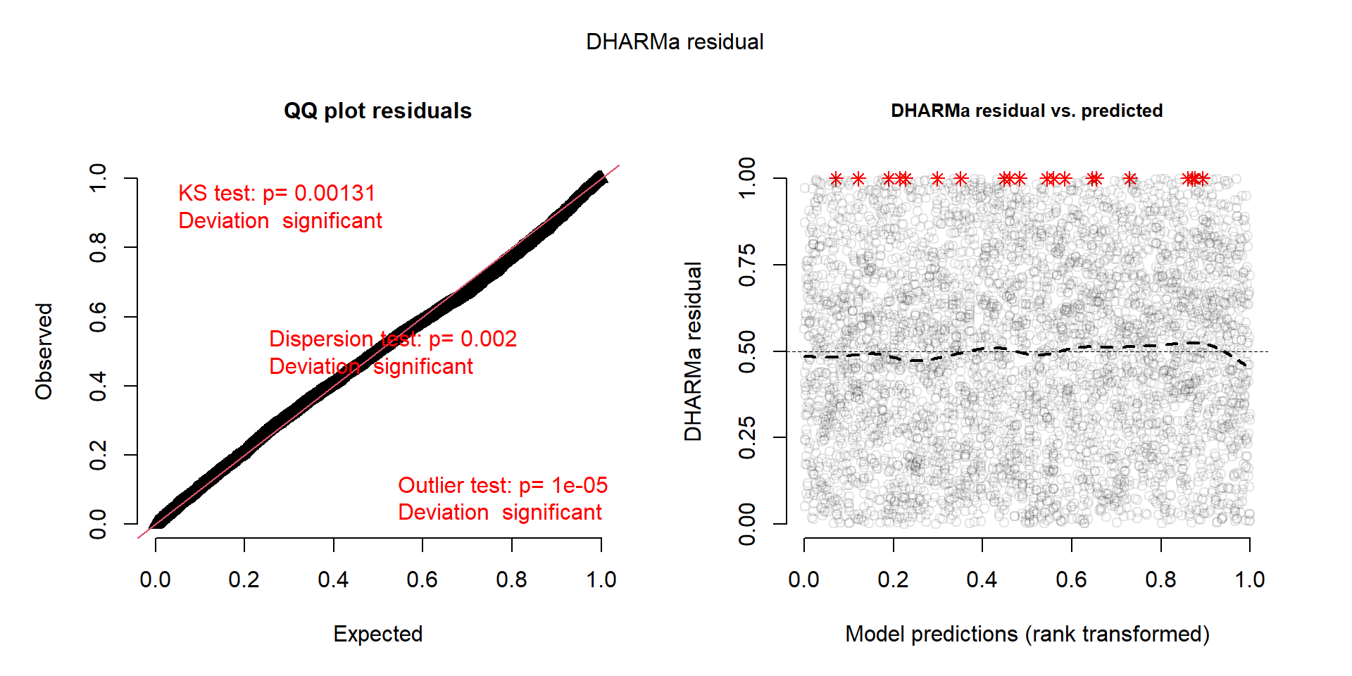
The QQ curve lies close to the diagonal, and the right-panel smoother stays near 0.5 through most of the fitted range. Across the 4,406 observations, the diagnostic statistics pick up small but consistent departures. The next checks trace those departures through the observed count frequencies and covariates.
NoteBootstrap outlier check
DHARMa calls an observation a simulation outlier when its observed count falls below or above every value simulated for that participant. Some such cases arise even under a well-fitting model, and their expected frequency depends on the number of simulations. For integer outcomes, the simple theoretical approximation can be inaccurate, so the bootstrap applies the same outside-the-simulated-range rule to data generated under the fitted model.
The testOutliers() reference recommends at least 1,000 simulations and 1,000 bootstrap replicates for integer-valued outcomes. Here the bootstrap estimates how often observations should fall beyond all their simulated values and compares that expectation with the observed frequency.
Show bootstrap outlier-test code
zinb_outlier_test <- testOutliers(
  zinb_residuals,
  type = "bootstrap",
  nBoot = 1000,
  plot = FALSE
)

outlier_table <- tibble::tibble(
  Quantity = c(
    "Observed counts beyond all simulated values",
    "Expected 95% frequency range under the fitted model",
    "Bootstrap comparison"
  ),
  Result = c(
    sprintf(
      "%d of %s (%.2f%%)",
      unname(zinb_outlier_test$statistic),
      format(
        unname(zinb_outlier_test$parameter),
        big.mark = ",",
        scientific = FALSE
      ),
      100 * unname(zinb_outlier_test$estimate)
    ),
    sprintf(
      "%.2f%%–%.2f%%",
      100 * unname(zinb_outlier_test$conf.int[1]),
      100 * unname(zinb_outlier_test$conf.int[2])
    ),
    paste(
      "p",
      if (zinb_outlier_test$p.value < 0.001) {
        "< 0.001"
      } else {
        paste("=", format.pval(zinb_outlier_test$p.value, digits = 2))
      }
    )
  )
)

knitr::kable(outlier_table, align = c("l", "l"))| Quantity | Result |
|---|---|
| Observed counts beyond all simulated values | 20 of 4,406 (0.45%) |
| Expected 95% frequency range under the fitted model | 0.05%–0.25% |
| Bootstrap comparison | p < 0.001 |
The compact ZINB produces 20 observations beyond the simulated range, compared with the much lower frequency expected under the fitted model. This result can arise from misspecified tails, unusual but valid observations, or data errors; the test does not distinguish among them. Individual records should be removed only when an independent data-quality check shows that they are invalid. Otherwise, they remain part of the evidence used to refine the model.
We next return from scaled residuals to the visit counts themselves. Figure 6 compares the observed frequency of each count with the range generated by the same simulations, using the earlier NB model as a benchmark.
Show count-frequency check code
summarise_count_frequencies <- function(residuals, model_name) {
  simulated <- residuals$simulatedResponse
  observed <- medcare$ofp
  displayed_counts <- 0:15
  count_labels <- c(as.character(displayed_counts), "16+")

  simulated_counts <- c(
    lapply(displayed_counts, function(value) {
      colSums(simulated == value)
    }),
    list(colSums(simulated >= 16))
  )

  tibble::tibble(
    Model = model_name,
    Count = factor(count_labels, levels = count_labels),
    Observed = c(
      vapply(
        displayed_counts,
        function(value) sum(observed == value),
        numeric(1)
      ),
      sum(observed >= 16)
    ),
    `Simulated median` = vapply(
      simulated_counts,
      median,
      numeric(1)
    ),
    Lower = vapply(
      simulated_counts,
      quantile,
      numeric(1),
      probs = 0.025,
      names = FALSE
    ),
    Upper = vapply(
      simulated_counts,
      quantile,
      numeric(1),
      probs = 0.975,
      names = FALSE
    )
  )
}

count_frequency_check <- bind_rows(
  summarise_count_frequencies(
    nb_residuals,
    "Negative-binomial benchmark"
  ),
  summarise_count_frequencies(
    zinb_residuals,
    "Compact ZINB"
  )
) |>
  mutate(
    Model = factor(
      Model,
      levels = c(
        "Negative-binomial benchmark",
        "Compact ZINB"
      )
    )
  )

ggplot(count_frequency_check, aes(x = Count)) +
  geom_linerange(
    aes(
      ymin = Lower,
      ymax = Upper,
      colour = "95% simulation interval"
    ),
    linewidth = 0.8
  ) +
  geom_point(
    aes(y = `Simulated median`, colour = "Simulated median"),
    shape = 95,
    size = 5
  ) +
  geom_point(
    aes(y = Observed, colour = "Observed frequency"),
    size = 2
  ) +
  facet_wrap(vars(Model), ncol = 1) +
  scale_colour_manual(
    values = c(
      "95% simulation interval" = "#5B8DB8",
      "Simulated median" = "#1F4E79",
      "Observed frequency" = "#B23A33"
    )
  ) +
  labs(
    x = "Physician office visits",
    y = "Number of participants",
    colour = NULL
  ) +
  theme_minimal(base_size = 11) +
  theme(
    legend.position = "bottom",
    panel.grid.minor = element_blank()
  )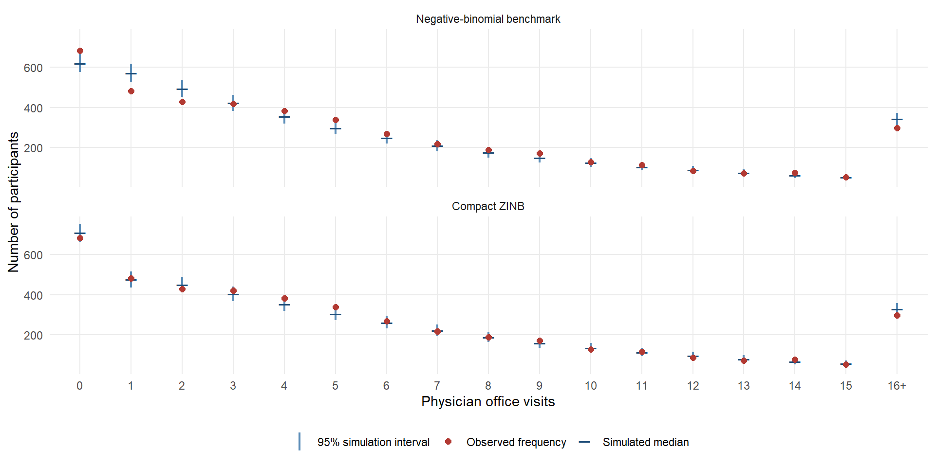
The NB panel shows the discrepancy already identified earlier: the observed zero count lies above its simulation interval, while counts of one and two are overproduced. The compact ZINB brings the zero and low-count frequencies much closer to the data. However, this marginal agreement can still conceal conditional problems because it pools participants with different fitted distributions.
To locate those problems, Figure 7 groups the ZINB residuals by age and chronic-condition count. A uniform residual distribution would place the three displayed quantiles on the dashed 0.25, 0.50, and 0.75 reference lines within every group.
Show covariate-residual check code
age_levels <- c(
  "66–69", "70–74", "75–79", "80–84", "85–89", "90+"
)
chronic_levels <- c("0", "1", "2", "3", "4", "5", "6+")

residual_covariates <- tibble::tibble(
  Residual = zinb_residuals$scaledResiduals,
  `Age band` = cut(
    round(medcare$age * 10),
    breaks = c(65, 69, 74, 79, 84, 89, Inf),
    labels = age_levels
  ),
  `Chronic conditions` = factor(
    ifelse(medcare$numchron >= 6, "6+", medcare$numchron),
    levels = chronic_levels
  )
)

age_quantiles <- residual_covariates |>
  group_by(`Age band`) |>
  summarise(
    Q25 = quantile(Residual, 0.25),
    Median = median(Residual),
    Q75 = quantile(Residual, 0.75),
    .groups = "drop"
  ) |>
  rename(Level = `Age band`)

chronic_quantiles <- residual_covariates |>
  group_by(`Chronic conditions`) |>
  summarise(
    Q25 = quantile(Residual, 0.25),
    Median = median(Residual),
    Q75 = quantile(Residual, 0.75),
    .groups = "drop"
  ) |>
  rename(Level = `Chronic conditions`)

to_long_quantiles <- function(data, panel_name) {
  bind_rows(
    transmute(
      data,
      Panel = panel_name,
      Level = as.character(Level),
      Quantile = "25th",
      Value = Q25
    ),
    transmute(
      data,
      Panel = panel_name,
      Level = as.character(Level),
      Quantile = "Median",
      Value = Median
    ),
    transmute(
      data,
      Panel = panel_name,
      Level = as.character(Level),
      Quantile = "75th",
      Value = Q75
    )
  )
}

covariate_quantiles <- bind_rows(
  to_long_quantiles(age_quantiles, "Age band (years)"),
  to_long_quantiles(chronic_quantiles, "Chronic conditions")
) |>
  mutate(
    Level = factor(Level, levels = c(age_levels, chronic_levels)),
    Quantile = factor(
      Quantile,
      levels = c("25th", "Median", "75th")
    )
  )

ggplot(
  covariate_quantiles,
  aes(x = Level, y = Value, colour = Quantile, group = Quantile)
) +
  geom_hline(
    yintercept = c(0.25, 0.5, 0.75),
    linetype = "dashed",
    colour = "#8A8A8A",
    linewidth = 0.5
  ) +
  geom_line(linewidth = 0.8) +
  geom_point(size = 2) +
  facet_wrap(vars(Panel), scales = "free_x", ncol = 2) +
  scale_colour_manual(
    values = c(
      "25th" = "#0072B2",
      "Median" = "#222222",
      "75th" = "#D55E00"
    )
  ) +
  scale_y_continuous(
    limits = c(0, 1),
    breaks = c(0, 0.25, 0.5, 0.75, 1)
  ) +
  labs(
    x = NULL,
    y = "DHARMa scaled-residual quantile",
    colour = "Within-group quantile"
  ) +
  theme_minimal(base_size = 11) +
  theme(
    legend.position = "bottom",
    panel.grid.minor = element_blank()
  )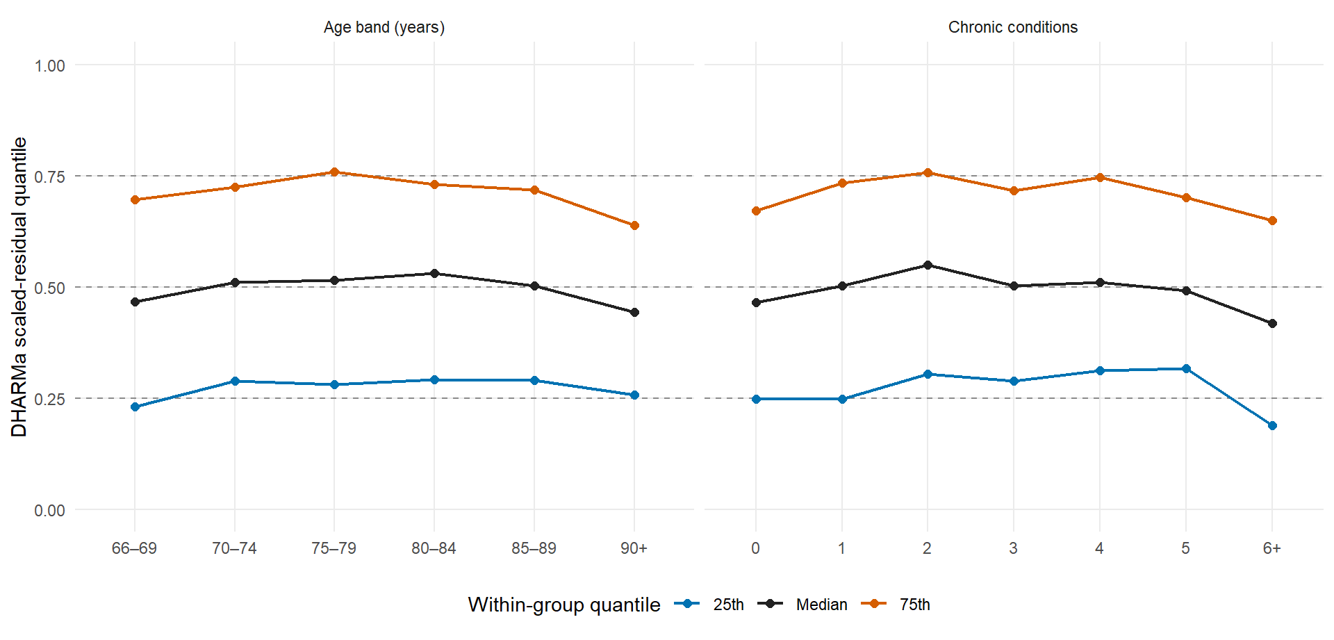
The age quantiles drift below their references among the oldest participants, rather than continuing the near-flat pattern implied by a single linear age term. Chronic-condition groups also vary, particularly at the low and high ends of the observed range. The plots locate the clearest departures in these parts of the data. Either the count mean, the extra-zero probability, or a combination of the two could produce the patterns.
The remaining binary predictors could hide group-specific departures or suggest an omitted interaction. Figure 8 therefore compares the residual distributions across health status, sex, and marital status. For uniform residuals, each box should have a median near 0.5 and its lower and upper edges near 0.25 and 0.75.
Show grouped-residual check code
health_status <- factor(
  ifelse(
    medcare$healthpoor == 1,
    "Poor",
    ifelse(medcare$healthexcellent == 1, "Excellent", "Average")
  ),
  levels = c("Average", "Poor", "Excellent")
)

group_residuals <- bind_rows(
  tibble::tibble(
    Panel = "Health status",
    Level = as.character(health_status),
    Residual = zinb_residuals$scaledResiduals
  ),
  tibble::tibble(
    Panel = "Sex",
    Level = ifelse(medcare$male == 1, "Male", "Female"),
    Residual = zinb_residuals$scaledResiduals
  ),
  tibble::tibble(
    Panel = "Marital status",
    Level = ifelse(
      medcare$married == 1,
      "Married",
      "Not married"
    ),
    Residual = zinb_residuals$scaledResiduals
  )
) |>
  mutate(
    Panel = factor(
      Panel,
      levels = c("Health status", "Sex", "Marital status")
    ),
    Level = factor(
      Level,
      levels = c(
        "Average", "Poor", "Excellent",
        "Female", "Male",
        "Not married", "Married"
      )
    )
  )

ggplot(group_residuals, aes(x = Level, y = Residual)) +
  geom_hline(
    yintercept = c(0.25, 0.5, 0.75),
    linetype = "dashed",
    colour = "#8A8A8A",
    linewidth = 0.5
  ) +
  geom_boxplot(
    fill = "#D9E8F5",
    colour = "#1F4E79",
    width = 0.62,
    outlier.alpha = 0.15,
    outlier.size = 0.7
  ) +
  facet_wrap(vars(Panel), scales = "free_x", ncol = 3) +
  scale_y_continuous(
    limits = c(0, 1),
    breaks = c(0, 0.25, 0.5, 0.75, 1)
  ) +
  labs(
    x = NULL,
    y = "DHARMa scaled residual"
  ) +
  theme_minimal(base_size = 11) +
  theme(panel.grid.minor = element_blank())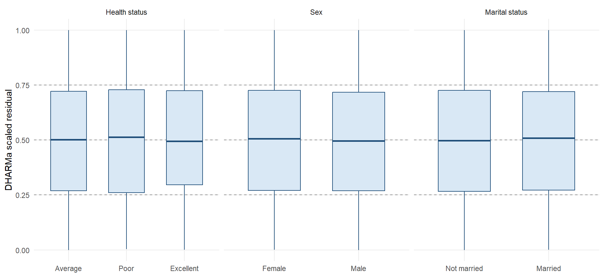
The group distributions are broadly similar, with no particular health, sex, or marital-status interaction standing out as the next addition. The age and chronic-condition patterns offer clearer directions for further work. A fuller analysis could compare substantively motivated nonlinear terms in the count mean, the extra-zero equation, or both, and evaluate them with out-of-sample data or resampling. Adding a quadratic term chosen from these same residual plots would instead combine model development and assessment in one step.
Together, these standard checks show that the compact ZINB reproduces the overall zero and low-count frequencies much better than the negative-binomial benchmark. The remaining departures are meaningful but limited in magnitude: residual spread is about 18% above its simulated expectation, the largest uniformity gap is 2.9 percentage points, and 20 of 4,406 observations (0.45%) fall beyond all their simulated values. The age and chronic-condition plots locate further discrepancies mainly at the ends of their observed ranges. The small p-values make these patterns unlikely to be simulation noise; their absolute size and location determine how much they matter in practice.
These results support a calculated working-model choice, and for the sake of this tutorial, I retain the compact ZINB as an illustrative working model because it is effectively tied for the lowest AIC, has the lowest BIC, repairs the main zero-frequency discrepancy, and directly represents the two-process question of interest. A fuller analysis would compare substantively motivated nonlinear terms, interactions, and alternative specifications, preferably with out-of-sample assessment. The next subsection interprets the fitted components while carrying these diagnostic limitations into the conclusions.
5.5 Interpreting the Zero-Inflated Model
A zero-inflated regression offers two related views of the fitted associations. We first examine \(\mu_i\) and \(\pi_i\) separately to see whether each predictor acts through the count-generating state, the latent extra-zero state, or both. We then recombine the two components on the observed response scale, where their associations may reinforce or offset one another. The first view explains how the model represents the data; the second gives the practical interpretation in expected visits.
5.5.1 Component-Specific Associations
Building on the regression formulation, we interpret the illustrative working model in two passes: \(\mu_i\), the conditional mean number of visits in the count-generating state, and \(\pi_i\), the probability assigned to the latent extra-zero state. Exponentiating their regression coefficients gives multiplicative associations with the count-component conditional mean and with the odds assigned to the extra-zero state, respectively.
Show count-component interpretation code
count_df <- model_parameters(
  zinb_model,
  component = "conditional",
  effects = "fixed",
  exponentiate = TRUE
) |>
  filter(Parameter != "(Intercept)") |>
  transmute(
    Predictor = recode(
      Parameter,
      healthpoor = "Poor vs average health",
      healthexcellent = "Excellent vs average health",
      numchron = "Chronic conditions (per condition)",
      age = "Age (per decade)",
      male = "Male vs female",
      married = "Married vs not married"
    ),
    `Conditional-mean ratio` = sprintf("%.2f", Coefficient),
    `95% CI` = sprintf("%.2f–%.2f", CI_low, CI_high),
    `p-value` = format.pval(p, digits = 2, eps = 0.001)
  )

knitr::kable(count_df, align = c("l", "r", "c", "r"), row.names = FALSE)| Predictor | Conditional-mean ratio | 95% CI | p-value |
|---|---|---|---|
| Poor vs average health | 1.32 | 1.21–1.44 | <0.001 |
| Excellent vs average health | 0.73 | 0.65–0.82 | <0.001 |
| Chronic conditions (per condition) | 1.16 | 1.14–1.19 | <0.001 |
| Age (per decade) | 0.95 | 0.90–0.99 | 0.027 |
| Male vs female | 0.98 | 0.91–1.05 | 0.485 |
| Married vs not married | 0.94 | 0.87–1.01 | 0.077 |
Show zero-inflation-component interpretation code
zi_df <- model_parameters(
  zinb_model,
  component = "zero_inflated",
  effects = "fixed",
  exponentiate = TRUE
) |>
  filter(Parameter != "(Intercept)") |>
  transmute(
    Predictor = recode(
      Parameter,
      healthpoor = "Poor vs average health",
      healthexcellent = "Excellent vs average health",
      numchron = "Chronic conditions (per condition)",
      age = "Age (per decade)",
      male = "Male vs female",
      married = "Married vs not married"
    ),
    `Odds ratio` = sprintf("%.2f", Coefficient),
    `95% CI` = sprintf("%.2f–%.2f", CI_low, CI_high),
    `p-value` = format.pval(p, digits = 2, eps = 0.001)
  )

knitr::kable(zi_df, align = c("l", "r", "c", "r"), row.names = FALSE)| Predictor | Odds ratio | 95% CI | p-value |
|---|---|---|---|
| Chronic conditions (per condition) | 0.28 | 0.19–0.41 | <0.001 |
| Male vs female | 3.08 | 1.84–5.16 | <0.001 |
| Married vs not married | 0.35 | 0.21–0.59 | <0.001 |
\(\mu_i\): within the count-generating state, the count-component conditional mean is 16% higher for each additional chronic condition (conditional-mean ratio 1.16, 95% CI 1.14–1.19) and 32% higher for poor rather than average health (1.32, 95% CI 1.21–1.44). Excellent rather than average health is associated with a 27% lower conditional mean (0.73, 95% CI 0.65–0.82), while each additional decade of age is associated with a 5% lower conditional mean (0.95, 95% CI 0.90–0.99). The estimates for sex and marital status are close to 1, and their confidence intervals include 1.
\(\pi_i\): each additional chronic condition is associated with 72% lower odds assigned to the latent extra-zero state (odds ratio 0.28, 95% CI 0.19–0.41). The fitted odds are higher for men than women (3.08, 95% CI 1.84–5.16) and lower for married participants than for participants who were not married (0.35, 95% CI 0.21–0.59). Here, the odds refer only to a modelled latent-state probability. Observed-zero odds and membership in a known patient group are different quantities.
It’s important to note that the reported intervals and p-values assume that the compact formula was fixed in advance, although its predictors were informed partly by observed-zero associations in these data. Specification selection therefore adds uncertainty beyond the reported coefficient estimates. We treat every association as a descriptive summary of the fitted specification, without a causal or individual-classification interpretation.
5.5.2 Overall Expected Visits
The component tables describe \(\mu_i\) and \(\pi_i\) separately, but neither component alone tells us how expected visits change. A predictor can shift the count mean, the extra-zero probability, or both; those shifts may reinforce or offset one another. We therefore combine them in the original outcome units as \((1-\pi_i)\mu_i\).
To see what the two pathways imply together, we create two versions of each eligible record. We change the predictor of interest, retain the observed values of every other predictor, and calculate overall expected visits for both versions. Averaging those predictions across the eligible records gives two standardized means; their difference and ratio form the standardized contrast reported in Table 14. We report three such comparisons:
- Sex and marriage: set the relevant binary indicator to 0 for every record in the reference version and to 1 in the comparison version.
- Chronic conditions: compare each eligible participant at their observed count and at one additional condition. Excluding the three participants already at the observed maximum of eight avoids extrapolating beyond the data and leaves 4,403 records.
Here, standardization refers to averaging record-level predictions over the observed covariate distribution. Every predictor remains on its original scale.
The scenario definitions and averaging operation specify the target quantities: a response-scale difference and ratio. We next quantify their sampling uncertainty. Both combine \(\mu_i\) and \(\pi_i\), so their intervals must carry uncertainty in the two components, including their covariance, through the nonlinear expression \((1-\pi_i)\mu_i\).
We use a full-refit parametric bootstrap. Each replicate treats the fitted compact ZINB as a data-generating model and follows three steps:
- simulate new visit counts at the observed covariate values,
- refit both model components,
- recalculate the same standardized differences and ratios.
CautionHow the contrasts and intervals are constructed
Let \(\mathcal I\) denote the records eligible for a contrast, and let \(\mathbf{x}_i^{(0)}\) and \(\mathbf{x}_i^{(1)}\) denote the reference and comparison versions of record \(i\). For the fitted ZINB, the overall expected count under version \(s\) is
\[ \widehat m_i^{(s)} = \left(1 - \widehat\pi_i^{(s)}\right)\widehat\mu_i^{(s)}. \]
Here, \(s=0\) identifies the reference version and \(s=1\) the comparison version.
Standardization averages these predictions over the eligible records:
\[ \overline{\widehat m}^{(s)} = \frac{1}{\lvert \mathcal I \rvert} \sum_{i \in \mathcal I} \widehat m_i^{(s)}. \]
The contrast is summarized as a difference and a ratio:
\[ \widehat\Delta = \overline{\widehat m}^{(1)} - \overline{\widehat m}^{(0)}, \qquad \widehat R = \frac{\overline{\widehat m}^{(1)}}{\overline{\widehat m}^{(0)}}. \]
For each bootstrap replicate, we simulate new outcomes from the fitted ZINB, refit the same count and zero formulas, and recalculate \(\widehat\Delta\) and \(\widehat R\). The 2.5th and 97.5th percentiles of the replicated values form the approximate 95% percentile parametric-bootstrap confidence intervals.
This simulate–refit–recalculate cycle estimates sampling uncertainty in the complete standardized contrast. Table 14 reports approximate 95% percentile intervals from 500 replicates.
Show prediction-scenario and contrast code
average_response_prediction <- function(model, newdata) {
  mean(predict(model, newdata = newdata, type = "response"))
}

# For chronic conditions, compare each eligible participant's observed count
# with that count plus one. Excluding the observed maximum avoids extrapolation.
chronic_reference <- medcare |>
  filter(numchron < max(numchron))
chronic_comparison <- chronic_reference |>
  mutate(numchron = numchron + 1)

# Binary contrasts compare two versions of every record while keeping the
# remaining observed predictors unchanged.
female_scenario <- medcare |>
  mutate(male = 0)
male_scenario <- medcare |>
  mutate(male = 1)
not_married_scenario <- medcare |>
  mutate(married = 0)
married_scenario <- medcare |>
  mutate(married = 1)

estimate_response_contrasts <- function(model) {
  tibble::tibble(
    Contrast_id = c("chronic", "sex", "marriage"),
    Contrast = c(
      "Adding one chronic condition among participants with 0–7 conditions",
      "Male vs female",
      "Married vs not married"
    ),
    Reference = c(
      average_response_prediction(model, chronic_reference),
      average_response_prediction(model, female_scenario),
      average_response_prediction(model, not_married_scenario)
    ),
    Comparison = c(
      average_response_prediction(model, chronic_comparison),
      average_response_prediction(model, male_scenario),
      average_response_prediction(model, married_scenario)
    )
  ) |>
    mutate(
      Difference = Comparison - Reference,
      Ratio = Comparison / Reference
    )
}

overall_point_contrasts <- estimate_response_contrasts(zinb_model)

# bootMer requires a numeric statistic. Stopping here records an unstable refit
# as a bootstrap failure rather than allowing it to enter the intervals.
bootstrap_response_statistic <- function(model) {
  fit_is_stable <-
    identical(model$fit$convergence, 0L) &&
    isTRUE(model$sdr$pdHess)

  if (!fit_is_stable) {
    stop("Bootstrap refit failed the convergence or Hessian check.")
  }

  contrasts <- estimate_response_contrasts(model)
  statistics <- c(contrasts$Difference, contrasts$Ratio)
  names(statistics) <- c(
    paste0(contrasts$Contrast_id, "_difference"),
    paste0(contrasts$Contrast_id, "_ratio")
  )
  statistics
}
Show parametric-bootstrap refit code
n_boot <- 500L
bootstrap_seed <- 20260730L

# Leave one physical core free for Quarto and other desktop work. The fallback
# keeps the tutorial runnable when R cannot determine the physical core count.
physical_cores <- parallel::detectCores(logical = FALSE)
n_workers <- if (is.na(physical_cores)) {
  1L
} else {
  max(1L, physical_cores - 1L)
}

run_bootstrap_refits <- function() {
  bootstrap_cluster <- parallel::makeCluster(n_workers)
  on.exit(parallel::stopCluster(bootstrap_cluster), add = TRUE)

  # Windows uses separate R sessions, so each worker needs the modelling
  # packages and every object used when glmmTMB reconstructs the original fit.
  parallel::clusterEvalQ(
    bootstrap_cluster,
    suppressPackageStartupMessages({
      library(lme4)
      library(glmmTMB)
      library(dplyr)
    })
  )

  parallel::clusterExport(
    bootstrap_cluster,
    c(
      "zinb_model", "medcare",
      "chronic_reference", "chronic_comparison",
      "female_scenario", "male_scenario",
      "not_married_scenario", "married_scenario",
      "average_response_prediction", "estimate_response_contrasts",
      "bootstrap_response_statistic"
    ),
    envir = environment()
  )

  # bootMer simulates outcomes, refits the complete ZINB, and evaluates the six
  # response-scale statistics for every replicate. Each refit uses one thread;
  # independent replicates are distributed across the worker processes.
  lme4::bootMer(
    zinb_model,
    FUN = bootstrap_response_statistic,
    nsim = n_boot,
    seed = bootstrap_seed,
    use.u = FALSE,
    type = "parametric",
    parallel = "snow",
    ncpus = n_workers,
    cl = bootstrap_cluster
  )
}

bootstrap_result <- run_bootstrap_refits()
bootstrap_succeeded <- complete.cases(bootstrap_result$t)
n_boot_success <- sum(bootstrap_succeeded)
n_boot_failed <- n_boot - n_boot_success
bootstrap_failure_messages <- attr(bootstrap_result, "boot.fail.msgs")

# A high failure rate makes percentile intervals unreliable and signals a model
# stability problem that should be investigated rather than silently ignored.
if (n_boot_success < 0.95 * n_boot) {
  stop(
    "Fewer than 95% of parametric-bootstrap models converged with ",
    "a positive-definite Hessian."
  )
}

# Cache only the raw successful statistics and diagnostics. Formatting remains
# in the lightweight table cell so prose or layout edits do not rerun refits.
bootstrap_statistics <- bootstrap_result$t[bootstrap_succeeded, , drop = FALSE]
rm(bootstrap_result)
Show interval-summary and table code
# Convert the cached bootstrap matrix into percentile intervals. This cell is
# intentionally lightweight: labels, rounding, and layout can change freely.
interval_endpoint <- function(column, probability) {
  quantile(
    bootstrap_statistics[, column],
    probs = probability,
    names = FALSE
  )
}

bootstrap_intervals <- tibble::tibble(
  Contrast_id = overall_point_contrasts$Contrast_id,
  Difference_low = vapply(
    paste0(Contrast_id, "_difference"),
    interval_endpoint,
    numeric(1),
    probability = 0.025
  ),
  Difference_high = vapply(
    paste0(Contrast_id, "_difference"),
    interval_endpoint,
    numeric(1),
    probability = 0.975
  ),
  Ratio_low = vapply(
    paste0(Contrast_id, "_ratio"),
    interval_endpoint,
    numeric(1),
    probability = 0.025
  ),
  Ratio_high = vapply(
    paste0(Contrast_id, "_ratio"),
    interval_endpoint,
    numeric(1),
    probability = 0.975
  )
)

overall_contrasts <- overall_point_contrasts |>
  left_join(bootstrap_intervals, by = "Contrast_id") |>
  transmute(
    Contrast,
    `Reference mean` = sprintf("%.2f", Reference),
    `Comparison mean` = sprintf("%.2f", Comparison),
    `Change (95% CI)` = sprintf(
      "%+.2f (%+.2f to %+.2f)",
      Difference,
      Difference_low,
      Difference_high
    ),
    `Ratio (95% CI)` = sprintf(
      "%.2f (%.2f–%.2f)",
      Ratio,
      Ratio_low,
      Ratio_high
    )
  )

knitr::kable(
  overall_contrasts,
  align = c("c", "c", "c", "r", "r"),
  row.names = FALSE
)| Contrast | Reference mean | Comparison mean | Change (95% CI) | Ratio (95% CI) |
|---|---|---|---|---|
| Adding one chronic condition among participants with 0–7 conditions | 5.79 | 6.97 | +1.18 (+1.02 to +1.36) | 1.20 (1.18–1.23) |
| Male vs female | 5.96 | 5.50 | -0.45 (-0.83 to -0.07) | 0.92 (0.86–0.99) |
| Married vs not married | 5.81 | 5.73 | -0.09 (-0.49 to +0.29) | 0.98 (0.92–1.05) |
The chronic-condition contrast uses 4,403 participants; the binary contrasts use all 4,406. Parentheses contain approximate 95% percentile parametric-bootstrap confidence intervals.
Adding one chronic condition is associated with 1.18 more expected visits (95% CI 1.02 to 1.36), or a 20% increase. The count-state mean rises while the estimated extra-zero probability falls, so both pathways reinforce the response-scale increase.
Men have 0.45 fewer expected visits than women after standardization (95% CI 0.07 to 0.83 fewer), an estimated reduction of 8%. Both component point estimates act in the same direction: the count-component mean is slightly lower for men, while their higher estimated extra-zero probability supplies most of the overall difference.
Married participants have 0.09 fewer expected visits than participants who are not married, but the interval ranges from 0.49 fewer to 0.29 more visits. Here the pathways oppose one another: the fitted count-state mean is lower for married participants, while their lower estimated extra-zero probability raises the response-scale expectation. The near cancellation leaves no clear overall difference under this specification.
NoteWhy use a parametric bootstrap?
A delta-method interval is a legitimate and much faster alternative. It approximates a nonlinear contrast with a straight line near the fitted coefficients and usually treats their joint sampling distribution as approximately normal. That approximation can work well, but our contrast averages a nonlinear combination of two fitted model components whose estimates can covary.
We chose the full-refit bootstrap because it carries that joint uncertainty through the complete calculation without first linearizing the contrast. Refitting also exposes simulated datasets in which the model cannot be estimated reliably. This choice is not universally superior: it costs more computation and still assumes that the fitted ZINB adequately represents the data-generating process. Readers who want to compare the delta method, coefficient simulation, and bootstrap approaches can consult the marginaleffects guide to uncertainty.
We use 500 replicates to keep the tutorial practical to reproduce. Substantive work should use more replicates when necessary and check that the interval endpoints are stable. The bootstrap used 5 local workers and successfully refitted 500 of 500 simulated datasets. The interval calculation excludes any refit that fails the convergence and Hessian checks used for the working model; none failed here.
The intervals condition on the observed covariates, the compact specification, and the fitted ZINB data-generating model. They exclude uncertainty from formula selection and residual misspecification, and they do not support a causal interpretation.
The three comparisons expose a general feature of zero-inflated regression: a predictor’s practical association emerges only after the count and zero pathways are recombined. Reinforcing pathways can magnify the response-scale association, while opposing pathways can nearly cancel even when both components appear meaningful. Standardized contrasts translate this latent two-process representation into the expected observed outcome that motivated the analysis.
6 Conclusion and Final Remarks
In summary, we worked through a sequential modelling exercise that I hope resembles how you might approach a similar count dataset in practice. We began with Poisson to establish a baseline for the conditional mean, variation, and zero frequency. Its severe overdispersion and 37 expected zeros, against 683 observed, pointed towards a more flexible count distribution. When counts vary far more than Poisson allows, NB2 is often a good candidate to try next. Here, it accounted for about 91% of zeros (623) through a single count process.
With most of the apparent zero excess captured by NB2, the next question was whether adding a separate zero component improved this stronger baseline. We saw that adding a constant extra-zero component added very little. The substantial improvement appeared when that probability was allowed to vary across patient characteristics. Expanding the compact formula with three additional predictors provided no meaningful improvement after accounting for the extra complexity, so we retained the smaller specification as the more focused way to explore the two-process hypothesis.
In conclusion, I believe that one of the biggest takeaways for this tutorial should be that when we are facing a dataset with a relatively high number of zeros in our response variable, we should start a sequence of progressive comparisons, beginning with the count distribution itself. Before adding a zero component, we should ask whether a count distribution with more realistic variation can already reproduce most of the excess zeros. Any remaining zero component then becomes a scientific hypothesis of its own, with predictors, assumptions, and diagnostic consequences. The compact ZINB gives that hypothesis an interpretable form for this tutorial, and what we gain is a clearer account of how two possible pathways may shape the observed outcome—and a clearer view of where that account remains incomplete.
6.1 A Repeatable Workflow
The approach we used for the Medicare data, and that I have used in practice, can be broken down and adapted to other count outcomes:
- Define the outcome and the processes that may generate it. Establish the observation window or exposure, decide what one count represents, and identify plausible reasons for both variation in the counts and the occurrence of zeros.
- Establish a count-family baseline. Begin with a simple count model, then use dispersion and residual checks to decide whether the count distribution needs more flexibility. A negative-binomial model is often a useful next candidate when Poisson variation is too restrictive.
- Test a basic extra-zero component. Within the selected count family, compare the ordinary model with a matched specification containing a constant extra-zero probability. This isolates whether a zero component adds enough to justify further development.
- Choose zero-component predictors deliberately. Use subject-matter knowledge and direct measures of the proposed zero-generating process whenever possible. When several formulas are plausible, compare a small candidate set with clear substantive interpretations.
- Check estimation stability. Confirm optimizer convergence, a positive-definite Hessian, finite standard errors, and the absence of extreme zero-component estimates before using fit statistics or residual diagnostics.
- Check the complete fitted distribution. Use simulation diagnostics to examine zero frequency, dispersion, overall distributional fit, residual patterns across important predictors, and observed versus predicted count frequencies. For predictive work, add repeated out-of-sample assessment with a distribution-sensitive score, such as held-out log predictive density or ranked probability score, alongside RMSE.
- Interpret the model in terms of the observed outcome. Explain the count and zero components separately, then recombine them on the response scale. Keep the interpretation conditional on the chosen specification, its remaining diagnostic departures, and the scientific meaning of the latent state.
6.2 Choosing an Appropriate Candidate
Given the workflow, you can use the table below to form a candidate set, then use matched comparisons, estimation checks, and simulation diagnostics to decide which specifications remain defensible. Note that the table covers only the four model families discussed in this article; other count distributions and hurdle-type specifications may also be worth considering!
| Model | Appropriate Candidate When | Reconsider When |
|---|---|---|
| Poisson | The conditional mean and variance are compatible (equidispersed), and simulations reproduce the zero frequency and tails | Residuals show overdispersion, underdispersion, a zero-frequency mismatch, or systematic patterns across predictors |
| Negative binomial (NB2) | Variation exceeds the Poisson assumption, and NB2 reproduces the residual spread, zero frequency, and tails without a separate zero component | Important zero-frequency, dispersion, tail, or predictor-specific departures remain |
| Zero-inflated Poisson (ZIP) | A separate extra-zero process has a defensible scientific interpretation, adding it improves distributional fit, and Poisson variation remains adequate within the count state | The count component remains overdispersed, the zero component is unstable, or its predictors lack a substantive interpretation |
| Zero-inflated negative binomial (ZINB) | NB2 variation is needed, and a substantively defensible zero component improves distributional fit beyond ordinary NB2 | NB2 already reproduces the relevant features, zero-component estimates are unstable, or important residual departures remain |
6.3 Scope and Reproducibility
These qualifications define the boundaries of the Medicare example. Age is recorded in decades: 6.6 represents 66 years, as confirmed by the fuller AER::NMES1988 documentation. The available data provide no participant-specific observation times, and the models include no exposure offset. We therefore treat each participant’s visit count as observed over the same one-year period, the 1987 NMES observation year, and compare counts under this common observation window.
Without the original survey-design variables, the estimates describe associations within the supplied sample under model-based uncertainty. They should not be interpreted as design-based population estimates for US Medicare beneficiaries.
NoteSoftware used for this article
- Runtime: R 4.6.0 and Quarto 1.10.18
- Modelling and diagnostics:
glmmTMB1.1.14, DHARMa 0.5.0,performance0.17.0,parameters0.29.1, andlme42.0-1 - Data and output:
catdata1.2.5,dplyr1.2.1,ggplot24.0.3,gridExtra2.3, andknitr1.51
6.4 Further Reading
- For the Medicare example and its original economic application, Deb and Trivedi develop a finite-mixture analysis of healthcare use among older adults (Deb and Trivedi 1997).
- For model fitting, Brooks and colleagues explain
glmmTMB’s parameterizations and its implementation of zero-inflated generalized linear models (Brooks et al. 2017). - For model checking, Hartig documents the simulation-based residuals and diagnostic tests provided by DHARMa (Hartig 2026).
- For a broader practical guide in R, Zeileis, Kleiber, and Jackman compare Poisson, negative binomial, hurdle, and zero-inflated regression (Zeileis et al. 2008).
- For the methodological foundations, Lambert introduces zero-inflated Poisson regression, while Mullahy develops modified count models and hurdle-style formulations (Lambert 1992; Mullahy 1986).
7 References
Brooks, Mollie E., Kasper Kristensen, Koen J. van Benthem, et al. 2017. “glmmTMB Balances Speed and Flexibility Among Packages for Zero-Inflated Generalized Linear Mixed Modeling.” The R Journal 9 (2): 378–400. https://doi.org/10.32614/RJ-2017-066.
Deb, Partha, and Pravin K. Trivedi. 1997. “Demand for Medical Care by the Elderly: A Finite Mixture Approach.” Journal of Applied Econometrics 12 (3): 313–36. https://www.jstor.org/stable/2285252.
Dobson, Annette J., and Adrian G. Barnett. 2018. An Introduction to Generalized Linear Models. 4th ed. CRC Press.
Hartig, Florian. 2026. DHARMa: Residual Diagnostics for Hierarchical (Multi-Level/Mixed) Regression Models. https://florianhartig.github.io/DHARMa/.
Lambert, Diane. 1992. “Zero-Inflated Poisson Regression, with an Application to Defects in Manufacturing.” Technometrics 34 (1): 1–14. https://doi.org/10.2307/1269547.
Liu, Lei, Ya Chen Tina Shih, Robert L. Strawderman, Daowen Zhang, Bankole A. Johnson, and Haitao Chai. 2019. “Statistical Analysis of Zero-Inflated Nonnegative Continuous Data: A Review.” Statistical Science 34 (2): 253–79. https://doi.org/10.1214/18-STS681.
McCullagh, Peter, and John A. Nelder. 1989. Generalized Linear Models. 2nd ed. Chapman; Hall.
Mullahy, John. 1986. “Specification and Testing of Some Modified Count Data Models.” Journal of Econometrics 33 (3): 341–65. https://doi.org/10.1016/0304-4076(86)90002-3.
Ospina, Raydonal, and Silvia L. P. Ferrari. 2012. “A General Class of Zero-or-One Inflated Beta Regression Models.” Computational Statistics & Data Analysis 56 (6): 1609–23. https://doi.org/10.1016/j.csda.2011.10.005.
Schauberger, Gunther, and Gerhard Tutz. 2025. catdata: Categorical Data. https://CRAN.R-project.org/package=catdata.
Zeileis, Achim, Christian Kleiber, and Simon Jackman. 2008. “Regression Models for Count Data in R.” Journal of Statistical Software 27 (8): 1–25. https://doi.org/10.18637/jss.v027.i08.
Footnotes
For a fuller treatment, McCullagh and Nelder (1989) give the classic mathematical account, while Dobson and Barnett (2018) provide a more introductory route through the same material.↩︎
There is actually a very cool connection between the Poisson and negative binomial distribution: suppose that instead of taking a fixed Poisson visit rate, we let each person’s rate vary according to a gamma distribution – perhaps due to unobserved heterogeneity between people as mentioned previously. It then turns out that averaging over those rates gives us the negative binomial distribution! You can check out this worked derivation if interested↩︎